Download

1 / 39
390 likes | 550 Views
Testing Planet Migration Theories by Observations of Transiting Exoplanetary Systems. University of Tokyo Norio Narita. 1/39. Contents. Introduction (15 min) Diversity of Extrasolar Planets Planet Migration Theories Motivation (10 min) Transits and the Rossiter-McLaughlin Effect

E N D
Testing Planet Migration Theoriesby Observations of TransitingExoplanetary Systems University of Tokyo Norio Narita 1/39
Contents • Introduction (15 min) • Diversity of Extrasolar Planets • Planet Migration Theories • Motivation (10 min) • Transits and the Rossiter-McLaughlin Effect • Recent Results (15 min) • Simultaneous Subaru / MAGNUM Observations • Analysis and Results • Conclusion and Future Prospects (3 min) • Significance of Our Results • New Targets and Prospects 2/39
Discovery of extrasolar planets The first extrasolar planet 51 Peg. b was discovered by radial velocity measurements in 1995. More than 200 extrasolae planets have been discovered so far. We can discuss statistics of their distribution. 3/39
Diversity of extrasolar planets Jupiter Semi-major axis – Planet minimum mass Distribution 4/39
Diversity of extrasolar planets hot Jupiters 1 AU (Close-up of the distribution) 5/39
Diversity of extrasolar planets Eccentric Planets Jupiter Semi-major axis – Eccentricity Distribution 6/39
How do they form? • Giant planets lie at ~0.1AU • should originally form at larger orbital distances • planetary migration to inner orbits • Eccentric planets are common • would have mechanisms of eccentricity excitation • How can we explain these features? • gravitational interactions with other bodies in protoplanetary disk 7/39
Planet migration theories • disk-planet interaction • “Type I & II migration” • resultant planets would not have large eccentricity • planet-planet interaction • “jumping Jupiter model” • have possibilities to produce large eccentricity • planet-binary companion interaction • “Kozai oscillation” in binary planetary systems • also have possibilities to produce large eccentricity • explain HD 80606 system (e=0.927, Wu & Murray 2003) 8/39
Type I & II migration • planetary cores form beyond the snow line • the cores interact with the surrounding disk • planets migrate inward due to torque exchange with the disk • Type I migration: less than ~10ME • Type II migration: more than ~10ME • damping eccentricities and also inclination Type II migration Type I migration (Leiden Observatory Group) 9/39
Jumping Jupiter model • giant planets interact with each other in multi-planet systems • leads to orbital instability • one planet is thrown into close-in orbit • the planet obtains eccentricity and inclination* Note *: this inclination is relative to the initial orbital plane 10/39
Jumping Jupiter model inclination eccentricity 90% of samples have inclination of more than 10 deg produce large eccentricities semi-major axis periastron periastron distance finally become semi-major axis by tidal evolution in hot region Marzari & Weidenschilling (2002) 11/39
Note: Tidal evolution • time scale for planetary orbit circularization • time scale for stellar spin/planetary orbit coplanarization s: star, p: planet, adopting values for HD 209458b as a typical case P: orbital/rotation period, k: tidal Love number, Q: tidal quality factor (cf. 6×10⁴ < QJup < 2×10⁶) Typically τcopl is much longer than τcirc Mardling (2007), Winn et al. (2005) 12/39
orbit 1: high eccentricity and inclination orbit 2: low eccentricity and inclination (at least 40 deg) star binary orbital plane companion Kozai mechanism • distant binary companion perturbs a planetary orbit • leads to “Kozai oscillation” • due to conservation of angular momentum • the planetary orbit oscillates high/low eccentricity/inclination • the planet migrates by tidal evolution 13/39
Kozai migration eccentricity periastron inclination Wu & Murray (2003) 14/39
Differences in outcomes • disk-planet interaction • negligible eccentricity and inclination • mainstream of migration theories • but cannot explain eccentric planets • planet-planet interaction • possible large eccentricity and inclination • subsequent tidal evolution damps eccentricity • would explain distribution of eccentric planets • planet-binary companion interaction • large eccentricity and inclination 15/39
Motivation • How can we test these theories by observations? • eccentricity and inclination are possible clues • but eccentricity may be damped within planets’ age • inclination (angle between initial and final orbital plane) would be a good diagnostic • Stellar spin axis would preserve initial orbital axis* • the inclination is equal to the stellar spin axis and the planetary orbital axis (spin-orbit alignment) • But can we observe/constraint spin-orbit alignments of exoplanetary systems? Note *: Assumption 16/39
Transiting extrasolar planets Planets pass in front of their host star. Charbonneau et al. (2000) periodic dimming in photometry The first transiting planet HD 209458b was reported in 2000. 17/39
What can we learn from transiting planets? • Radial Velocity • semi-major axis a, minimum mass Mp sin i • Period P, eccentricity e • Transit Photometry • orbital inclination* iorb、radius ratio Rp/Rs • by combining spectroscopy: radius Rp, density ρ • Secondary Eclipse • thermal emission of planetary surface • Transmission Spectroscopy • search for atmospheric components • Na, H, C, O, H2O, SiO detections were reported in HD 209458b • (Subaru observations for HD 189733b tomorrow) Note *: this inclination is relative to the sky plane 18/39
Radial Velocity during Transit Transiting planet hides stellar rotation. star planet planet hide approaching side → appear to be receding hide receding side → appear to be approaching Radial velocity would have anomalous excursion during transit. 19/39
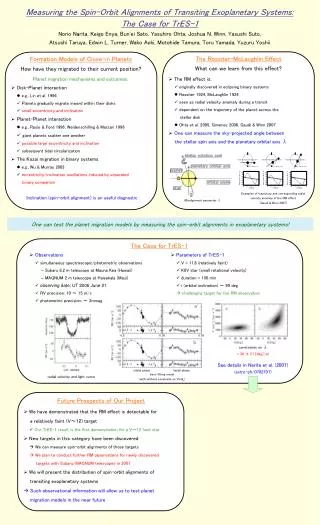
The Rossiter-McLaughlin effect This effect was originally reported in eclipsing binary systems. β Lyrae: Rossiter 1924, ApJ, 60, 15 Algol: McLaughlin 1924, ApJ, 60, 22 20/39
RM effect in transiting exoplanetary system ELODIE on 193cm telescope Queloz et al. (2000) The RM effect was detected in HD 209458b in 2000. 21/39
What can we learn from the RM effect? RV anomaly time examples of trajectory Ohta, Taruya & Suto (2005) Radial velocity anomaly reflects planet’ trajectory. 22/39
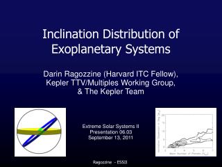
Definition of λ λ: sky-projected angle between the stellar spin axis and the planetary orbital axis 23/39
Planetary trajectories and λ We can measure λ by observations of the RM effect. Gaudi & Winn (2007) 24/39
Summary of introduction and motivation • There are several different planet migration theories. • Each theory has different distributions of eccentricity and inclination. • We can observe the RM effect in transiting exoplanetary systems. • We can measure λ(sky-projected spin-orbit alignment) via the RM effect. • λ is an useful diagnostic for testing planet migration theories. A B E C D 25/39
Our recent observations Brief summary Target : TrES-1 (V=11.8) → the faintest target so far Observation : Simultaneous Subaru/MAGNUM observations Challenge : the first RM observation for Subaru & MAGNUM Result : succeeded in detection of the RM effect and placed a constraint on λ Significance 1: extended targets of the RM observations to fainter systems Significance 2: discovery of a possible misaligned system 26/39
Backgrounds of the RM observations History of discoveries of target systems before 2005 HD 209458 : 2000, V=7.65 TrES-1 : 2004, V=11.8 HD 149026 : 2005, V=8.15 HD 189733 : 2005, V=7.67 … The RM observations were conducted for brighter targets with Keck/HIRES HD 209458 : Winn et al. 2005 HD 189733 : Winn et al. 2006 (HD 149026 : Wolf et al. 200?) 27/39
Possible targets of the RM observations Possible targets → Transiting systems brighter than V~12 (for which we can detect the RM effect with Subaru/HDS) Our target : TrES-1, V=11.8 The first challenge for a fainter (V~12) target (also the first RM observation for Subaru/HDS) 28/39
TrES-1 • Discovered with 10cm telescope (Alonso et al. 2004) • V=11.8、K0V、V sin Is = 1.08 ± 0.30 km/s) • Poor radial velocity measurements due to its faintness. • The star has several spots. Upper:TrES-1 Lower:HD 209458 ※Charbonneau et al. (2007) 29/39
Simultaneous Subaru/MAGNUM observations TrES-1 observations with 2 telescopes in Hawaii (UT 2006/6/21) Photometry with MAGNUM at Haleakala Radial velocity measurement with Subaru/HDS 30/39
20 samples R : 45000 Exposure time : 15 min Seeing : ~1.0 arcsec S/N : ~ 60 (with iodine cell) Radial velocity analysis by Sato et al. (2002) RV precision : 10 ~ 15 m/s RV measurements with Subaru/HDS Radial velocities obtained with Subaru/HDS 31/39
Photometry with MAGNUM • 184 samples • Band : V • Exposure time : 40 or 60 sec • No spot event • Photo. precision : 2 mmag • Timing precision : ~30 sec V band transit light curve obtained with MAGNUM 32/39
RV model and parameters • incorporating published data • Keck 12 ( 7 + 5 ) RV samples • FLWO 1149 (3 transits) photometric samples • RM modeling with Ohta, Taruya, & Suto formula(2005) • Simultaneous fitting of radial velocity and photometry • including the RM effect • 15 free parameters • K, VsinIs, λ : for radial velocity • iorb, uV, uz, Rs, Rp/Rs : for photometry • v1, v2, v3 : offsets for radial velocity datasets • Tc(234), Tc(235), Tc(236), Tc(238) : time of transit center 33/39
(a) (b) Note: Constraints on VsinIs • External constraint on VsinIs for TrES-1 • VsinIs = 1.08 ± 0.30 km/s (Laughlin et al. 2005) • Fitting with (a) / without (b) considering the constraint • χ2 minimization with AMOEBA (Numerical Recipes) 34/39
Results of RV fitting 0 0 -0.5 0.05 orbital phase transit phase a : with, b : without 35/39
Constraints on VsinIs and λ (a) : VsinIs = 1.3 ± 0.3 [km/s], λ= 30 ± 21 [deg] (b) : VsinIs = 2.5 ± 0.8 [km/s], λ= 48 ± 17 [deg] Contours : ⊿χ2=1,00, ⊿χ2=2.30, ⊿χ2=4.00, ⊿χ2=6.17 36/39
Summary of Our Recent Results • We detected the RM effect in TrES-1 (V~12) • TrES-1 is the faintest target so far • We confirm that similar observations are possible for other faint systems • We put a constraint on λ in TrES-1 for the first time • large uncertainty, but at least we confirmed that the planet orbits in a prograde manner • possible misaligned (over 10 deg) system • additional RM observations would pin down λ • the first candidate of the jumping Jupiter model 37/39
What’s next? New targets were discovered in 2006 & 2007 • 4 ground-based transit survey teams (XO, TrES, HAT, WASP) succeeded in detecting new transiting systems • all transit survey teams target V less than ~12 • also ESA’s satellite mission (CoRoT) started in 2007 • 2006 : XO-1, TrES-2, HAT-P-1, WASP-1, WASP-2 • 2007 : CoRoT-1, TrES-3, XO-2, XO-3, HAT-P-2, GJ 436 • (recent news) : XO-4, TrES-4, HAT-P-3, HAT-P-4, more to come! observational / statistical studies have become possible 38/39
Future Prospects • We can measure the RM effect of new transiting systems • By measuring the distribution of spin-orbit alignment, we can test planet migration theories • already we have • possible misaligned target TrES-1 → further constraint on λ • at least 15 new targets • We can present observational / statistical distribution of spin-orbit alignment within several years 39/39