Download
1 / 46
460 likes | 477 Views
This article provides an introduction to decision trees, explaining their structure, advantages, and how they are used for classification and regression. It also covers pruning techniques and the extraction of rules from decision trees.

E N D
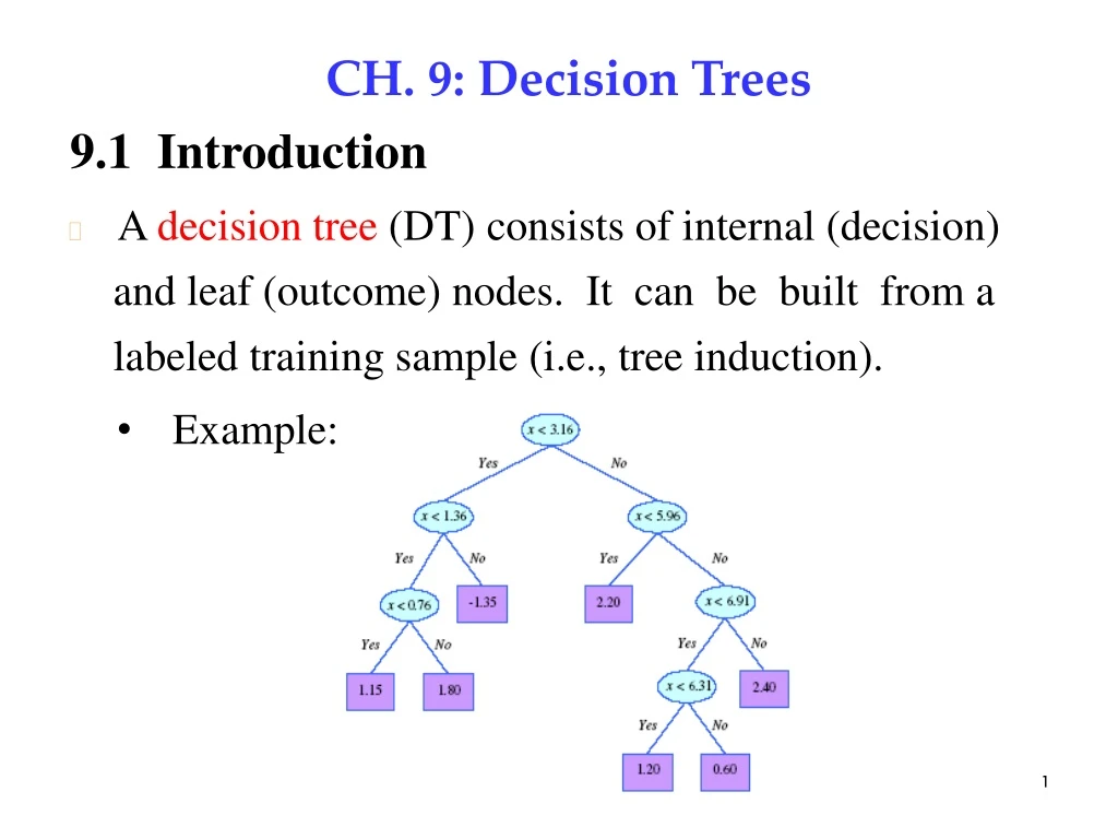
9.1 Introduction CH. 9: Decision Trees • A decision tree (DT) consists of internal (decision) and leaf (outcome) nodes. It can be built from a labeled training sample (i.e., tree induction). • Example: 1
Each decision node goes with a test function with discrete outcomes labeling branches. Each leaf node has a class label (for classification) or a numeric value (for regression). • A leaf node defines a localized region in the data space. Within the region, instances belong to the same class or have similar values. The boundaries of the region are determined by the discriminants that coded in the internal nodes on the path from the root to the leaf node. 2
Example: In a 2D data space, • Example: The leaf nodes define hyperrectangles in the input space. 3
Advantages of DT (a) A DT represents a function F (x) returning a label (classification) or a value (regression) (b) A DT can be represented as a set of IF-THEN rules that are easily understandable 9.2 Univariate Trees • In a univariate tree, each internal node makes a decision based on only one attribute. In a multivariate tree, each internal node makes a decision based on multiple attributes. 4
A tree learning algorithm starts at the root with the • complete training data. At each step, it looks for the • best split of the subset of training data corresponding • to the node under consideration based on a chosen • attribute. It continues until no split is needed and a • leaf node is created. • The goodness of a split is quantified by an impurity measure. In practice, the smaller the measure, the better the split. 5
Consider 2-class case and is an impurity measure function if Examples: 1.Entropy: 6
For K-class case, When , is largest. 2. Gini index: 3. Misclassification error: 9.2.1 Classification Trees • Given a training set, many trees can code it. Objective: Find the smallest one. • Tree size is measured by: • i) # nodes, ii) the complexity of decision nodes. 7
N : # training instances Nm : # instances reachingnode m fm : test function at m nm : # branched from m : # instances along branch j # instances belonging to class K : # classes probability of an instancereaching m belonging to 8
Node ispure if are either 0 or 1. only one of the probabilities is 1 and the others are all 0 ) A leaf node labeled with the class for which can be added. The split associated with a pure node is called pure, in which all the instances choosing a branch belong to the same class; no further split is necessary. 9
If node m is pure, generate a leaf and stop, otherwise split and continue recursively Impurity after split: of Nm take branchj. belong to Ci Total impurity: CART Algorithm: • For all attributes, calculate their split impurity and choose the one with the minimum impurity. 10
Difficulties with the CART Algorithm: 1. Splitting favors attributes with many values many values many branches less impurity Methods have to balance the impurity drop and the branching factor. Noise may lead to a very large tree if highly pure tree is desired. Methods reduce tree complexities by introducing thresholds for impurity measures of nodes and probabilities of creating leaf nodes. 11
9.2.2 Regression Trees during constructing a tree, the goodness of a split of a node is measured by the mean square error with the estimated mean value. Considering node m, let Xm: the subset of X reaching node m The mean square error (MSE): 13
where If the error is acceptable, i.e. , a leaf node is created and value is stored. Otherwise, data reaching node m is split further such that the sum of the errors in the branches is minimized. 14
: the subset of Xmtaking branch j Let nm : # branched at node m : the estimated value in branch j of node m The total MSE after splitting: We look for the split that is minimum. 15
The CART algorithm can be modified to training a regression tree by replacing (i) entropy with mean square error and (ii) class labels with averages. • Another possible error function: • Worst possible error 16
A small error thresh leads to a large tree and overfit. • Example: Different wrong correct 17
9.3 Pruning • Two types of pruning: Prepruning: Early stopping, e.g., small number of examples reaching a node Postpruning: Grow the whole tree then prune unnecessary subtrees that cause overfitting 20 * Prepruning is faster, postpruning is more accurate
9.4 Rules Extraction from Trees Example: During building a univariate tree,certain features (e.g., ) may not be used. Features (e.g., ) closer to the root are more important. A decision node carries a condition. Each path from the root to a leaf corresponds to one conjunction of tests and can be written down a set of IF-THEN rules. 21
Example: IF-Then Rules: Rule support – the percentage of training data covered by the rule 22
Multiple conjunctive expressions correspond to different paths can be combined as a disjunction. Example: 23
9.5 Learning Rules from Data • Two ways to get rules: Tree induction – trains a decision tree and converts it to rules Rule induction – learns rules directly from data • Differences between these two ways: Tree induction conducts breadth-first search and generates all paths simultaneous Rule induction performs depth-first search and generates one path (rule) at a time 24
Each rule is a conjunction of conditions, which are added one at a time, to optimize some criterion. A rule is said to cover an example if the example satisfies all the conditions of the rule. Sequential covering: Once a rule is grown, it is added to the rule base and all the training examples covered by the rule are removed. The process continues until enough rules are added. E.g., Ripper: a rule induction algorithm 25
9.6 Multivariate Trees At a decision node m, all input dimensions can be used to split the node. When all inputs are numeric, Linear multivariate node: 28
Quadratic multivariate node: Sphere node: 29
Summary • A decision tree (DT) consists of internal (decision) and leaf (outcome) nodes. Each decision node goes with a test function. Each leaf node has a class label or a numeric value. • Types of DT • Univariate tree -each internal node makes a decision based on only one attribute. Multivariate tree - each internal node makes a decision based on multiple attributes. 30
A tree learning algorithm starts at the root with the • complete training data. At each step, it looks for the • best split of the subset of training data based on a • chosen attribute. It continues until no split is needed • and a leaf node is created. • The goodness of a split is quantified by an impurity measure, e.g., 1.Entropy: 2. Gini index: 3. Misclassification error: 31
For K-class case, When , is largest. 2. Gini index: 3. Misclassification error: 9.2.1 Classification Trees • Given a training set, many trees can code it. Objective: Find the smallest one. • Tree size is measured by: • i) # nodes, ii) the complexity of decision nodes. 34
Appendix: Entropy • In information theory, • let probability of occurrence If e occurs, we receive bits of information. Bit: the amount of information receives when any of two equally probable alternatives is observed, This means that if we know for sure that an event will occur, its occurrence provides no information at all. 37
。 Consider a sequence of symbols output from the source with occurring probabilities Zero-memory source: the probability of sending each symbol is independent of symbols previously sent. The amount of information received from each symbol is Entropy of the information source: the average amount of information received per symbol 38
。 Entropy measures the degree of disorder of a system. The most disorderly system is the one whose symbols occur with equal probability. Proof: The difference in entropy between the two sources 39
The second term in (1) is zero where informationgain (relative entropy or Kullback-Leibler divergence between and ) 41
In statistical mechanics – Systems deal with ensembles, each of which contains a large number of identical small systems, e.g., thermodynamics, quantum mechanics -- The property of an ensemble is determined by the average behavior of constituent small systems. Example: A thermodynamic system that is initially at temperature is changed to T 42
At temperature T, sufficient time should be given in order to allow the system to reach an equilibrium, in which the probability that a particle i has an energy following the Boltzmann distribution T : Kelvins temperature where : Boltzmann constant The system energy at the equilibrium state ( ) is in an average sense . 43
: Partition function 。 The coarseness of particle i with energy : The entropy of the system is the average coarseness of its constituent particles 44
○ Two systems with the respective entropies Suppose they have the same energy, i.e., Suppose follows Boltzmann distribution, i.e., The entropy difference between two systems 45
* A system whose constituent small systems with their energy follow the Boltzmann distribution has the largest entropy. 46


![9.1 Introduction [1/3]](https://cdn2.slideserve.com/4796852/9-1-introduction-1-3-dt.jpg)