Recursive Algorithms: Definition, Types, and Examples
770 likes | 795 Views
This article explains the definition of recursive algorithms and their properties. It also discusses the different types of recursion, such as direct, indirect, tail, linear, and tree recursion. Examples of factorial computations using recursion are provided.

Recursive Algorithms: Definition, Types, and Examples
E N D
Presentation Transcript
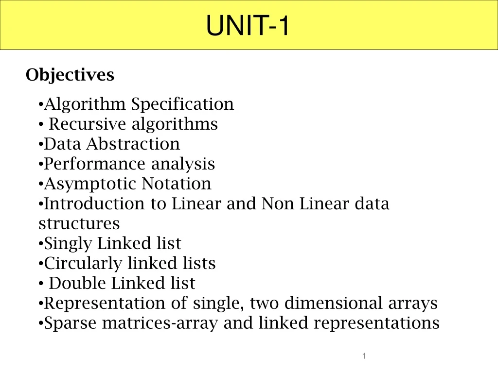
UNIT-1 Objectives <number>
ALGORITHM Definition: An Algorithm is a method of representing the step-by-step procedure for solving a problem. It is a method of finding the right answer to a problem or to a different problem by breaking the problem into simple cases. It must possess the following properties: Finiteness: An algorithm should terminate in a finite number of steps. Definiteness: Each step of the algorithm must be precisely (clearly) stated. Effectiveness: Each step must be effective.i.e; it should be easily convertible into program statement and can be performed exactly in a finite amount of time. Generality: Algorithm should be complete in itself, so that it can be used to solve all problems of given type for any input data. Input/Output: Each algorithm must take zero, one or more quantities as input data and gives one of more output values. <number>
Recursive Algorithms 1 of 10 <number>
Recursive Algorithms 2 of 10 All recursive algorithms must obey three important laws: A recursive algorithm must have a base case. A recursive algorithm must change its state and move toward the base case. A recursive algorithm must call itself, recursively Types of Recursions: Direct Recursion Indirect Recursion Tail Recursion Linear Recursion Tree Recursion <number>
Recursive Algorithms 3 of 10 1. Direct Recursion A C function is directlyrecursiveif it contains an explicit call to itself Int foo (int x) { if ( x <= 0 ) return x; return foo ( x – 1); } <number>
Recursive Algorithms 4 of 10 2. Indirect Recursion A C function foo1 is indirectlyrecursive if it contains a call to another function that ultimately calls foo1. int foo1(int x){ if (x <= 0) return x; return foo2 (x); } int foo2 (int y) { return foo1(y – 1); } <number>
Recursive Algorithms 5 of 10 3. Tail Recursion A recursive function is said to be tail recursive if there is no pending operations performed on return from a recursive call Tailrecursive functions are often said to “return the value of the last recursive call as the value of the function” Tail recursive factorial int fact_Trec (int n, int result) { if (n == 1) return result;return fact_Trec (n – 1, n * result); } factorial (int n) { return fact_Trec (n, 1); } factorial is non-tail recursive int factorial (int n) { if (n == 0) return 1; return n * factorial(n – 1); } Note: The “pending operation” (namely the multiplication) to be performed on return from each recursive call <number>
Recursive Algorithms 6 of 10 4. Linear Recursion A recursive function is said to be linearly recursive when no pending operation invokes another recursive call to the function. int factorial (int n) { if (n == 0) return 1; return n * factorial ( n – 1); } <number>
Recursive Algorithms 7 of 10 5.Tree Recursion A recursive function is said to be tree recursive (or non-linearly recursive when the pending operation does invoke another recursive call to the function. The Fibonacci function fib provides a classic example of tree recursion. // Note how the pending operation (the +) // needs a 2nd recursive call to fib int fib(int n) { if (n == 0) return 0; if (n == 1) return 1; return ( fib ( n – 1 ) + fib ( n – 2 ) ); } <number>
Recursive Algorithms 8 of 10 Example1 : Factorial (Recursion) Compute the factorial of integer n: n! = 1 2 · · · n = ( 1 n = 1 n (n − 1)! n > 1 algorithm factorial(n) if n = 1 then return 1 // base case of the recursion else return n factorial(n − 1) // recursive call The execution of a recursive algorithm uses a call stack to keep track of previous method call <number>
Recursive Algorithms 9 of 10 Example 2: Factorial (Tail-Recursion) The previous factorial algorithm is augmented recursive, i.e. it can be replaced by a tail-recursion <number>
Recursive Algorithms 10 of 10 Example 3: Factorial (Iteration) The tail-recursive factorial algorithm can be replaced by a simple iterative loop <number>
Data Abstraction The basic data types includes char , int , float & double. Some data types may be modified by keywords short , long , unsigned Two mechanisms for grouping data together: Arrays Structures Data types: It is a collection of objects & set of operations that act on those objects. int consists of objects { 0 , +1 , -1 , +2 , -2 , INT_MAX, INT_MIN } INT_MAX : largest integer on machine INT_MIN: smallest integer on machine It includes in <limits.h> <number>
Data Abstraction Abstract Data Type(ADT): It is a data type i.e, organised in such a way that the specification of the objects & the specification of the operations on the objects is separated from the representation of the objects & implementation of the operations. e.g : Ada have packages C++ have class The functions of a data types into several categories: Creator / constructor Transformers Observers / reporters <number>
Data Abstraction Creator / constructor: These functions create a new instance of the designed type. 2. Transformers : These functions also create an instance of the designed type generally by using 1 / more other instances. 3. Observers / reporters: These functions provide information about an instance of the type , but they do not change the instance <number>
PERFORMANCE ANALYSIS 1 of 4 <number>
PERFORMANCE ANALYSIS 2 of 4 <number>
PERFORMANCE ANALYSIS 3 of 4 <number>
PERFORMANCE ANALYSIS 4 of 4 Example:1 Algorithm add(a,b,c) { return a+b+c; } If we assume a, b, c occupy one word size then total size comes to be 3 S(p) = C (since C=3) Example:2 Algorithm add(x,n) { sum=0.0; for i= 1 to n do sum:=sum+x[i]; return sum; } The n space required for x[], one space for n, one for i, and one for sum S(p) ≥ (n+3) <number>
Asymptotic Notations: 1 of 5 <number>
Asymptotic Notations: 2 of 5 Big Oh Notation Big Oh notation denoted by ‘O’ is a method of representing the upper bound of algorithm’s running time. Using big oh notation we can give longest amount of time taken by the algorithm to complete. Definition: Let, f(n) and g(n) are two non-negative functions. And if there exists an integer n0 and constant C such that C > 0 and for all integers n > n0, f(n) ≤ c*g(n), then f(n) = Og(n). Various meanings associated with big-oh are O(1)constant computing time O(n)linear O(n2)quadratic O(n3)cubic O(2n)exponential O(logn)logarithmic The relationship among these computing time is O(1)< O(logn)< O(n)< O(nlogn)< O(n2)< O(2n) <number>
Asymptotic Notations: 3 of 5 Omega Notation Omega notation denoted ‘Ω’ is a method of representing the lower bound of algorithm’s running time. Using omega notation we can denote shortest amount of time taken by algorithm to complete. Definition: Let, f(n) and g(n) are two non-negative functions. And if there exists an integer n0 and constant C such that C > 0 and for all integers n > n0, f(n) >c*g(n), then f(n) = Ω g(n). <number>
Asymptotic Notations: 4 of 5 Theta Notation Theta notation denoted as ‘θ’ is a method of representing running time between upper bound and lower bound. Definition: Let, f(n) and g(n) are two non-negative functions. There exists positive constants C1 and C2 such that C1 g(n) ≤ f(n) ≤ C2 g(n) and f(n) = θ g(n) <number>
Asymptotic Notations: 5 of 5 <number>
Introduction to Linear & Non-linear Data Structure 1 of 3 The data structure can be defined as the collection of elements and all the possible operations which are required for those set of elements. In other words data structure will tell us specific set of elements and corresponding set of operations. A data structure can be defined as a way of organizing and storing data in a computer so that it can used efficiently. Mathematically, a data structure D is a triplet, that is, D=(d, f, a) where D= data structure d= a set of variables (data objects) f= a set of functions a= set of rules to implement the functions. <number>
Introduction to Linear & Non-linear Data Structure 2 of 3 Data Structures: A data structure is an arrangement of data in a computer's memory or even disk storage. It classified into two types Linear Data Structures Non Linear Data Structures 1. Linear Data Structures: Linear data structures are those data structures in which data elements are accessed (read and written) in sequential fashion ( one by one) Eg: Stacks , Queues, Lists, Arrays 2. Non Linear Data Structures: Non Linear Data Structures are those in which data elements are not accessed in sequential fashion. Eg: trees, graphs <number>
Introduction to Linear & Non-linear Data Structure 3 of 3 Types of Data Structure Data Structure Primitive Data Structures Non Primitive Data Structures Eg: int, char, float Linear Data Structures Non Linear Data Structures Eg: array, linked list, stack, queue Eg: trees, graphs <number>
Difference between linear and non linear data structures <number>
Difference between linear and non linear data structures <number>
Difference between linear and non linear data structures <number>
SINGLY LINKED LIST 1 of 14 <number>
SINGLY LINKED LIST 2 of 14 NODE node struct Node { int data; struct Node *link; }; link data LINKED LIST Start Null A B C D <number>
SINGLY LINKED LIST 3 of 14 <number>
SINGLY LINKED LIST 4 of 14 <number>
SINGLY LINKED LIST 5 of 14 <number>
SINGLY LINKED LIST 6 of 14 <number>
SINGLY LINKED LIST 7 of 14 CREATION OF A NODE: Inittially first=NULL last=NULL struct node *cur; cur=(struct node*)malloc(size of(struct node)); Read cur->data cur->link=NULL <number>
SINGLY LINKED LIST 8 of 14 Algorithm for creating a node Step 1: if the list is empty then first==NULL Step 2: Create a new node cur= (struct node*) malloc (sizeof (struct node)); Step 3: Read the content of node Step 4: Assign new node link to NULL cur->link=NULL Step 5: Assign new node to first & last node first=cur last=cur Step 6: If the list is not empty call insert function insert () Step 7 : Stop <number>
SINGLY LINKED LIST 9 of 14 <number>
SINGLY LINKED LIST 10 of 14 Case 1 : at the beginning Pseudo code: Inserting at beginning of list. if (first! = NULL) { Cur=(struct node*) malloc (sizeof(struct node)) Read cur->data Cur->lnk=first First=cur } <number>
SINGLY LINKED LIST 11 of 14 Case 2 : end of the list <number>
SINGLY LINKED LIST 12 of 14 Case 3 : after a given element Pseudo code: Inserting at end of list. if (first! = NULL) { Cur=(struct node*) malloc (sizeof(struct node)) Read cur->data Next=first while(next!=NULL) { if(next->data = = key) break; else next=next->link; } cur -> link = next->link; next->link = cur; } <number>
SINGLY LINKED LIST 12 of 14 Case 4 : Before a given element <number>
SINGLY LINKED LIST 12 of 14 DELETION: Removing an element from the list, without destroying the integrity of the list itself. When we delete a node we logically remove the node from the list by changing links and physically remove it from heap 1)deletion from beginning of list 2)deletion at middle of list 3)deletion at end of list <number>
SINGLY LINKED LIST 13 of 14 DELETION at the beginning of list: Pseudo code: While(curr!=NULL) if(curr->data = = key) break; else prev=curr; curr=curr->next; if(curr==header) header = curr->next; else prev->next = curr->next; delete curr; <number>
SINGLY LINKED LIST 14 of 14 TRAVERSAL: Pseudo code: temp = header; while(temp!=NULL) cout<<temp->data; temp = temp->next; C program example1 , also show error simulation <number>
CIRCULARLY LINKED LIST A circularly linked list, or simply circular list, is a linked list in which the last node is always points to the first node. This type of list can be build just by replacing the NULL pointer at the end of the list with a pointer which points to the first node. There is no first or last node in the circular list. Advantages: Any node can be traversed starting from any other node in the list. There is no need of NULL pointer to signal the end of the list and hence, all pointers contain valid addresses. In contrast to singly linked list, deletion operation in circular list is simplified as the search for the previous node of an element to be deleted can be started from that item itself. <number>
CIRCULARLY LINKED LIST Insertion at the front of Circular linked list Procedure for insertion a node at the beginning of list Step1. Create the new nodeStep2. Set the new node’s next to itself (circular!) Step3. If the list is empty, return new node.Step4. Set our new node’s next to the front.Step5. Set tail’s next to our new node. Step6. Return the end of the list. <number>
CIRCULARLY LINKED LIST Insertion in the middle of the Circular linked list <number>
CIRCULARLY LINKED LIST Insertion at the end of Circular linked list Procedure for insertion a node at the end of list Step1. Create the new nodeStep2. Set the new node’s next to itself (circular!) Step3. If the list is empty,return new node.Step4. Set our new node’s next to the front.Step5. Set tail’s next to our new node. Step6. Return the end of the list. <number>
