Download

1 / 30
300 likes | 412 Views
X-ray variability of 104 active galactic nuclei XMM-Newton power-spectrum density profiles. Authors: O.Gonzalez-Martin, S. Vaughan Speaker: Xuechen Zheng 2014.5.13. Outline. Introduction Sample and Data Data Analysis Results Discussion. Introduction. Introduction.

E N D
X-ray variability of 104 active galactic nuclei XMM-Newton power-spectrum density profiles Authors: O.Gonzalez-Martin, S. Vaughan Speaker: Xuechen Zheng 2014.5.13
Outline • Introduction • Sample and Data • Data Analysis • Results • Discussion
Introduction • 1、PSD: BH-XRB vs. AGN • Similarities: power law, bend frequency • BH-XRB: ‘state’– PSD shape • QPOs problem • 2、Main purpose: • AGN PSD properties
Sample and Data • From XMM-Newton public archives until Feb. 2009: • Z <0.4 • Observation duration T >40 ksec • Classification, redshift, mass, bolometric luminosity: literature • Sample: 209 observations and 104 distinct AGN(61 Type-1, 21 Type-2, 15 NLSy1, 7 BLLACs)
2 – 10 keV luminosity • 2-10 kev luminosity fitting using absorbed power-law model • Required only reasonable estimates • LLAGN luminosity agree with other literature • Type- 1 Seyferts, QSOs, NLSy1:high discrepancies soft-excess long-term variability
PSD estimation • For a given PSD model P(ν;θ), likelihood function: • I: observed P: model • Confidence intervals:
Two models • A. Simple power law: • B. Bending power law:
Select model • LRT: Likelihood ratio test • Not well calibrated • Accurate calibration: computation expensive
QPOs check • 1、Largest outlier vs. Chi-squared distribution for periodogram • Candidate: p<0.01 • 2、Similar test to smoothing periodogram (top-hat filter) • QPOs broader than frequency resolution • p-value not correctly calibrated, crude but efficient
Result 1 - variability • 75 out of 104 AGN show variability • No variability: 12 of 14 LINERs, 2 of 11 Type-2 Seyferts, 12 of 54 Type-1 Seyferts, 2 of 3 QSOs, 1 of 7 BLLACs
Result 2 -- Model selection • Low number of bins in the PSD above Poisson noise some sources unable to constrained parameters • Model B: 17 • vs. Papadakis et al.(2010): bump or QPOs? • 16 Type-1, 1 S2
Result 3 • QPOs: only one candidate • Slope: • Model A ---- α=2.01±0.01(T) 2.06±0.01(S) 1.77±0.01(H) • K-S test distributions statistically indistinguishable • Model B ---- α=3.08±0.04(T) 3.03±0.01(S) 3.15±0.08(H)
Result 4 – bend frequency • Mean value: log(v_b) = -3.47 ± 0.10
Result 5 – bend amplitude • Papadakis(2004): A=ν×F(ν) roughly constant at bend frequency
Result 6 -- Leakage • Leakage bias: reduce sensitivity to bends and QPOs • model A α≈ 2: possibly be affected • ‘End matching’(Fougere 1985) reduce leakage bias • remove linear trend: first and last point equal • model A indices higher than before but lower than high frequency index in bend PSDs
Result summary • 1、72% of the sample show variability, most LINERs do not vary • 2、17 sources (16 Type-1 Seyferts) model B; others model A • 3、slope discrepancy between model A and B • 4、only one QPO (hard to detect)
Scaling relation • Equation 1: • A = 1.09 ±0.21 C = -1.70 ±0.29 • SSE :11.14 for 19 dof • Equation 2: • A = 1.34 ±0.36 B = -0.24 ±0.28 • C = -1.88 ±0.36 • SSE: 10.69 for 18 dof
Scaling relation • Cygnus X-1: test relation on BH-XRB • vs. McHardy et al.(2006): • Weak dependence of T_b on L • Use smaller mass dependence recover( B = -0.70 ±0.30) • Maybe due to uncertainties
BLR vs. variability • McHardy et al.(2006): correlation between T and optical line widths(V) • Lines: Hβ, Paβ • Correlation coefficient: r = 0.692 • D = 2.9 ±0.7 E = -10.2±2.3 • SSE: 13.47 for 19 dof
PSD shapes • Model B high frequency slope steep: • May be similar to BH-XRB‘soft’states • XMM-Newton and RXTE • Selection effect • Majority of sample show no bend: • Massive object have lower v_b • Leakage bias • selection effect • Bends: • M_bh, L expected T_b 17 source bends within frequency range(13 detected)