Download
1 / 51
510 likes | 647 Views
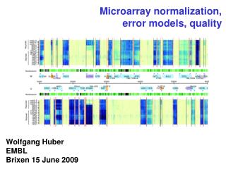
Microarray normalization and error models Wolfgang Huber European Bioinformatics Institute. H. Sueltmann DKFZ/MGA. Why do you need normalisation?. From: lymphoma dataset vsn package Alizadeh et al., Nature 2000. PCR plates. Scatterplot, colored by PCR-plate

E N D
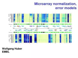
Microarray normalization and error models Wolfgang Huber European Bioinformatics Institute H. Sueltmann DKFZ/MGA
From: lymphoma dataset vsn package Alizadeh et al., Nature 2000
PCR plates Scatterplot, colored by PCR-plate Two RZPD Unigene II filters (cDNA nylon membranes)
print-tip effects F(q) q (log-ratio)
spotting pin quality decline after delivery of 5x10⁵ spots after delivery of 3x10⁵ spots H. Sueltmann DKFZ/MGA
spatial effects R Rb R-Rbcolor scale by rank another array: print-tip color scale ~ log(G) color scale ~ rank(G) spotted cDNA arrays, Stanford-type
Batches: array to array differences dij = madk(hik -hjk) arrays i=1…63; roughly sorted by time
A complex measurement process lies between mRNA concentrations and intensities The problem is less that these steps are ‘not perfect’; it is that they vary from array to array, experiment to experiment.
log-ratio Which genes are differentially transcribed? same-same tumor-normal
Statistics 101: biasaccuracy precision variance
Basic dogma of data analysis Can always increase sensitivity on the cost of specificity, or vice versa, the art is to - optimize both - then find the best trade-off. X X X X X X X X X
3000 3000 x3 ? 1500 200 1000 0 ? x1.5 A A B B C C But what if the gene is “off” (below detection limit) in one condition? ratios and fold changes Fold changes are useful to describe continuous changes in expression
ratios and fold changes The idea of the log-ratio (base 2) 0: no change +1: up by factor of 21 = 2 +2: up by factor of 22 = 4 -1: down by factor of 2-1 = 1/2 -2: down by factor of 2-2 = ¼ A unit for measuring changes in expression: assumes that a change from 1000 to 2000 units has a similar biological meaning to one from 5000 to 10000. What about a change from 0 to 500? - conceptually - noise, measurement precision
How to compare microarray intensities with each other? How to address measurement uncertainty (“variance”)? How to calibrate (“normalize”) for biases between samples? Questions
Systematic Stochastic o similar effect on many measurements o corrections can be estimated from data o too random to be ex-plicitely accounted for o remain as “noise” Calibration Error model Sources of variation amount of RNA in the biopsy efficiencies of -RNA extraction -reverse transcription -labeling -fluorescent detection probe purity and length distribution spotting efficiency, spot size cross-/unspecific hybridization stray signal
Error models • describe the possible outcomes of a set of measurements • Outcomes depend on: • true value of the measured quantity • (abundances of specific molecules in biological sample) • measurement apparatus • (cascade of biochemical reactions, optical detection system with laser scanner or CCD camera)
Error models • Purpose: • Data compression: summary statistic instead of full empirical distribution • Quality control • Statistical inference: appropriate parametric methods have better power than non-parametric (this has practical, financial, andethical aspects)
bi per-sample normalization factor bk sequence-wise probe efficiency hik ~ N(0,s22) “multiplicative noise” ai per-sample offset eik ~ N(0, bi2s12) “additive noise” The two component model measured intensity = offset + gain true abundance
“multiplicative” noise “additive” noise The two-component model raw scale log scale B. Durbin, D. Rocke, JCB 2001
Parameterization two practically equivalent forms (h<<1)
Important issues for model fitting Parameterization variance vs bias "Heteroskedasticity"(unequal variances) weighted regression or variance stabilizing transformation Outliers use a robust method Algorithm If likelihood is not quadratic, need non-linear optimization. Local minima / concavity of likelihood?
Models are never correct, but some are useful True relationship: Model: linear dependence Model: quadratic dependence
variance stabilizing transformations Xu a family of random variables with EXu=u, VarXu=v(u). Define var f(Xu ) independent of u derivation: linear approximation
1.) constant variance (‘additive’) 2.) constant CV (‘multiplicative’) 3.) offset 4.) additive and multiplicative variance stabilizing transformations
the “glog” transformation - - - f(x) = log(x) ———hs(x) = asinh(x/s) P. Munson, 2001 D. Rocke & B. Durbin, ISMB 2002 W. Huber et al., ISMB 2002
generalized log-ratio difference log-ratio variance: constant part proportional part glog raw scale log glog
Parameter estimation o maximum likelihood estimator: straightforward – but sensitive to deviations from normality o model holds for genes that are unchanged; differentially transcribed genes act as outliers. o robust variant of ML estimator, à la Least Trimmed Sum of Squares regression. o works well as long as <50% of genes are differentially transcribed (and may still work otherwise)
Least trimmed sum of squares regression minimize P. Rousseeuw, 1980s - least sum of squares - least trimmed sum of squares
“usual” log-ratio 'glog' (generalized log-ratio) c1, c2are experiment specific parameters (~level of background noise)
Variance-bias trade-off and shrinkage estimators Shrinkage estimators: pay a small price in bias for a large decrease of variance, so overall the mean-squared-error (MSE) is reduced. Particularly useful if you have few replicates. Generalized log-ratio: = a shrinkage estimator for fold change There are many possible choices, we chose “variance-stabilization”: + interpretable even in cases where genes are off in some conditions + can subsequently use standard statistical methods (hypothesis testing, ANOVA, clustering, classification…) with less worries about heteroskedasticity than with many alternative methods
“Single color normalization” • n red-green arrays (R1, G1, R2, G2,… Rn, Gn) • within/between slides • for (i=1:n) • calculate Mi= log(Ri/Gi), Ai= ½ log(Ri*Gi) • normalize Mi vs Ai • normalize M1…Mn • all at once • normalize the matrix of (R, G) • then calculate log-ratios or any other contrast you like
What about non-linear effects o Microarrays can be operated in a linear regime, where fluorescence intensity increases proportionally to target abundance (see e.g. Affymetrix dilution series) Two reasons for non-linearity: oAt the high intensity end:saturation/quenching. This can and should be avoided experimentally - loss of data! oAt the low intensity end:background offsets, instead of y=k·x we have y=k·x+x0, and in the log-log plot this can look curvilinear. But this is an affine-linear effect and can be correct by affine normalization. Non-parametric methods (e.g. loess) risk overfitting and loss of power.
Definitions linear affine linear genuinely non-linear
Bioinformatics and computational biology solutions using R and Bioconductor, R. Gentleman, V. Carey, W. Huber, R. Irizarry, S. Dudoit, Springer (2005). Variance stabilization applied to microarray data calibration and to the quantification of differential expression. W. Huber, A. von Heydebreck, H. Sültmann, A. Poustka, M. Vingron. Bioinformatics 18 suppl. 1 (2002), S96-S104. Exploration, Normalization, and Summaries of High Density Oligonucleotide Array Probe Level Data. R. Irizarry, B. Hobbs, F. Collins, …, T. Speed. Biostatistics 4 (2003) 249-264. Error models for microarray intensities. W. Huber, A. von Heydebreck, and M. Vingron. Encyclopedia of Genomics, Proteomics and Bioinformatics. John Wiley & sons (2005). Differential Expression with the Bioconductor Project. A. von Heydebreck, W. Huber, and R. Gentleman. Encyclopedia of Genomics, Proteomics and Bioinformatics. John Wiley & sons (2005). References
Anja von Heydebreck (Darmstadt) Robert Gentleman (Seattle) Günther Sawitzki (Heidelberg) Martin Vingron (Berlin) Annemarie Poustka, Holger Sültmann, Andreas Buness, Markus Ruschhaupt (Heidelberg) Rafael Irizarry (Baltimore) Judith Boer (Leiden) Anke Schroth (Heidelberg) Friederike Wilmer (Hilden) Acknowledgements
Genechip S. cerevisiae Tiling Array 4 bp tiling path over complete genome (12 M basepairs, 16 chromosomes) Sense and Antisense strands 6.5 Mio oligonucleotides 5 mm feature size manufactured by Affymetrix designed by Lars Steinmetz (EMBL & Stanford Genome Center)
Probe specific response normali-zation S/N 3.22 3.47 4.04 remove ‘dead’ probes 4.58 4.36
Probe-specific response normalization siprobe specific response factor. Estimate taken from DNA hybridization data bi =b(si )probe specific background term. Estimation: for strata of probes with similar si, estimate b through location estimator of distribution of intergenic probes, then interpolate to obtain continuous b(s)
Estimation of b: joint distribution of (DNA, RNA) values of intergenic PM probes unannotated transcripts log2 RNA intensity b(s) background log2 DNA intensity