Download

1 / 44
460 likes | 638 Views
Belief Networks (BRML ch. 3). Ishii Lab., Systems Science Department, Graduate School of Informatics, Uji Campus, Kyoto University Sequential Data Analysis Study Group By: Kourosh Meshgi To: SDA Study Group, Dr. Shigeyuki Oba On: 2011-11-11. Contents. The Benefits of Structure

E N D
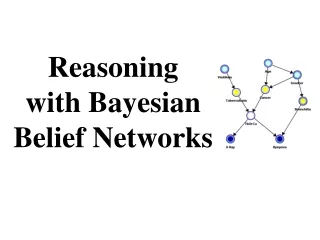
Belief Networks(BRML ch. 3) Ishii Lab., Systems Science Department, Graduate School of Informatics, Uji Campus, Kyoto University Sequential Data Analysis Study Group By: Kourosh Meshgi To: SDA Study Group, Dr. Shigeyuki Oba On: 2011-11-11
Contents • The Benefits of Structure • Uncertain and Unreliable Evidence • Belief Networks • Causality • Summary Kourosh Meshgi, SDA Study Group
Importance • Independently specifying all the entries of a table needs exponential space • Computational tractability of inferring quantities of interest • Idea: • to constrain the nature of the variable interactions • to specify which variables are independent of othersleadingto a structured factorisation of the joint probability distribution Kourosh Meshgi, SDA Study Group
Belief Networks • Also: Bayes' networks, Bayesian belief networks • A way to depict the independence assumptions made in a distribution • Application examples • Troubleshooting • Expert reasoning under uncertainty • Machine learning Kourosh Meshgi, SDA Study Group
Approach: Modeling • Read the problem • Make a model of the world • Variables (binary) • Probability distribution on the joint set of the variables of interest • Decomposition: Repeatedly using the definition of conditional probability • Lots of states (2 ^ # of variables) to be specified! Kourosh Meshgi, SDA Study Group
Independence Assumptions • Assume the A is not directly influenced by B • p(A|B) = p(A) • p(A|B,C) = p(A|C), … • Represent these conditional independencies graphically • What causedwhat? • e.g. R caused T • Reduces the number of values that we need to specify Kourosh Meshgi, SDA Study Group
Approach: Modeling (continue) • Read the problem • Make a model of the world • Decomposition • Conditional Independency Graph • Simplification: Simplify conditional probability terms of independent events Kourosh Meshgi, SDA Study Group
Inference • Bayes Rule • p(A|B) = p(A,B) / p(B) • p(A happens given that B happened): Posterior • B: Evidence • p(B): Prior knowledge about B • Calculate the probability model of the world • General purpose algorithms for this calculations • Junction Tree Algorithm Kourosh Meshgi, SDA Study Group
Explain Away • When additional evidence come to the calculation and cause the initial probability to drop dramatically, it is told that it explains away the first probability. • e.g. Alarm p( Burglar|A) = 0.99 Radio p( Burglar| A , R ) = 0.01 Knowing R drops p(B|<Evidence>) It explains away the chance of Burlgary Kourosh Meshgi, SDA Study Group
Reducing the burden of specification • Too much parents for each node? • Exponential # of rows in specification table • e.g. 32 rows for 5 binary parents • Solutions: • Constrain the table to have a simpler parametric form (e.g. Divorcing Parents) • Using simple classes of conditional tables (e.g. Noisy Logic gates) Kourosh Meshgi, SDA Study Group
Divorcing Parents • Constrain the table to have a simpler parametric form • Decomposition in which only a limited number of parental interactions are required • e.g. 16 (8 + 4 + 4) rows for 5 binary parents Kourosh Meshgi, SDA Study Group
Noisy Logic Gates • Using simple classes of conditional tables • The number of parameters required to specify the noisy gate is linear in the number of parents • Noisy-OR: at least one of the parents is present, the probability that the node will be present is high • e.g. 10 (=2+2+2+2+2) rows for 5 binary parents • disease-symptom networks Kourosh Meshgi, SDA Study Group
Uncertain (Soft) Evidence • The evidence variable is in more than one state, with the strength of our belief about each state being given by probabilities • In contrast, for hard evidence we are certain that a variable is in a particular state • e.g. p(A) → p(A | Ã) • Inference using Bayes' rule • Jeffrey’s Rule: first define the model conditioned on the evidence, and then average over the distribution of the evidence • a generalization of hard-evidence Kourosh Meshgi, SDA Study Group
Unreliable (Likelihood) Evidence • The evidence can’t be trusted 100%. • Virtual Evidence: own interpretation of the evidence. • e.g. p(A|B) → p(H | B) Kourosh Meshgi, SDA Study Group
Approach: Modeling • Read the problem • Make a model of the world • Decomposition • Conditional Independency Graph • Simplification • Substitute Unreliable Evidence with Virtual Ones • Jeffrey’s Rule • Adding Uncertain Evidence Kourosh Meshgi, SDA Study Group
Belief Networks Definition • A distribution of the form • Representation • Structure: Directed Acyclic Graph (DAG) • Arrows: Pointing from parent variable to child variable • Nodes: p(xi | pa(xi)) Kourosh Meshgi, SDA Study Group
Construction of BN on variables • Write down the n-node cascade graph • Label the nodes with the variables in any order • Each successive independence statement corresponds to deleting one of the edges. • Result: DAG Kourosh Meshgi, SDA Study Group
Notes • Every probability distribution can be written as a BN, even though it may correspond to a fully connected ‘cascade’ DAG. • The particular role of a BN is that the structure of the DAG corresponds to a set of conditional independenceassumptions, namely which parental variables are sufficient to specify each conditional probability table. • Non-parental variables do have influence BN shows which ancestors are direct ‘causes’for the variable. The ‘effects’, given by the descendants of the variable, will generally be dependent on the variable. Markov Blanket • After having DAG Specification of all Conditional Probability Tables(CBTs) is required. Kourosh Meshgi, SDA Study Group
Markov Blanket • In Bayesian network, the Markov Blanket of Node A includes its parents, children and the other parents of all of its children. • Carries all information about A • All dependency relations of A • MB (A) Kourosh Meshgi, SDA Study Group [Courtesy of Wikipedia.com]
Collision • Path P, Node c, Neighbor nodes a and b on P: • a → c ← b c is a collider • A collider is path specific (i.e. is defined relative to a path) • z is collider? Kourosh Meshgi, SDA Study Group
Independence using Collision • A non-collider zwhich is conditioned along the path between x and y cannot induce dependence between x and y. • A path between xand ywhich contains a collider & collider is not in the conditioning set (and neither are any of its descendants) this path does not make x and y dependent. • A path between x and ywhich contains no colliders and no conditioning variables this path ‘d-connects’ x and y. • x and y are independent? Kourosh Meshgi, SDA Study Group Graphically Conditionally Dependent
Example a ╨e | b ? a ╨e | c ? Kourosh Meshgi, SDA Study Group
A╨B ? p(A,B,C) = p(C|A,B)p(A)p(B) p(A,B,C) = p(A|C)p(B|C)p(C) Graphically Dependent Marginalization Kourosh Meshgi, SDA Study Group Conditioning Independent
Example 1 • C╨A ? • C ╨ A|B? • C ╨ D? • C ╨ D|A? • E ╨ C|D? • Any two variables are independent if they are not linked by just unknown variables. A B D C E Kourosh Meshgi, SDA Study Group
Example 2 • A╨E ? • A ╨ E|B? • A╨ E|C? • A ╨ B? • A ╨ B|C? • Don’t forget the explain away effect! A B C Kourosh Meshgi, SDA Study Group D E
In Other Words: In/Active Triplets Active Triplets Render variables dependent Inactive Triplets Render variables independent Kourosh Meshgi, SDA Study Group : Known Evidence
Example 3 • F╨A ? • F ╨ A|D? • F ╨ A|G? • F ╨ A|H? • Use shading the known technique. A C F B E H D Kourosh Meshgi, SDA Study Group G
Blocked Path of Dependence (z is given) • If there is a collider not in the conditioning set (upper path) we cut the links to the collider variable. In this case the upper path between x and y is ‘blocked’. • If there is a non-collider which is in the conditioning set (bottom path), we cut the link between the neighbors of this non-collider which cannot induce dependence between x and y. The bottom path is ‘blocked’. • In this case, neither path contributes to dependence. Both paths are ‘blocked’. Kourosh Meshgi, SDA Study Group
D-Separation & D-connection • G is a DAG, X & Y & Z are disjoint sets in G • X and Y are d-connected by Z in Giff There exist an undirected path U between some vertex in X and some vertex in Y such that for every collider C on U, either C or a descendent of C is in Z, and no non-collider on U is in Z. • X and Y are d-separatedby Z in Giffthey are not d-connected. • If all paths between X and Y are blocked then X and Y are d-separated by Z in G. • A path U is said to be blocked if there is a node w on U such that either • w is a collider and neither w nor any of its descendants is in Z, or • w is not a collider on U and w is in Z. Kourosh Meshgi, SDA Study Group
Bayes Ball Algorithm • Linear Time Complexity • Given X and Z • Determines the set of nodes, Y, such that X╨Y|Z. • Y is called the set of irrelevant nodes for X given Z. • Remember:X and Y are d-separated if there is no active path between them. Kourosh Meshgi, SDA Study Group
Bayes Ball Algorithm:The Ten Rules of Bayes Ball • An undirected path is active if a Bayes ball travelling along it never encounters the “stop”: • If there are no active paths from X to Y when {Z1, . . . ,Zk} are shaded, then X╨Y | {Z1, . . . ,Zk}. Kourosh Meshgi, SDA Study Group
Independence Using d-Separation • If the variable sets X and Y are d-separated by Z, they are independent conditional on Z in all probability distributions such a graph can represent. • If X and Y are d-connected by Z it doesn’t mean that X and Y are dependent in all distributions consist with the belief network structure. Kourosh Meshgi, SDA Study Group
Markov Equivalence • Two graphs are Markov equivalent if they both represent the same set of conditional independence statements. • This definition holds for both directed and undirected graphs. • Example • A→C←B CI statements: { A╨B|Ø } • A→C←B and A→C CI statements: { } • { A╨B|Ø } ≠ { } these BNs are not Markov equivqlent. Kourosh Meshgi, SDA Study Group
Determining Markov Equivalence • Immorality in DAG: A configuration of three nodes, A, B, C such that C is a child of both A and B, with A and B not directly connected. • Skeleton of Graph: Result of removing the directions on the arrows. • Markov Equivalence: Two DAGs represent the same set of independence assumptions if and only if they have the same skeleton and the same set of immoralities. Kourosh Meshgi, SDA Study Group
Example: Markov Equivalent? Kourosh Meshgi, SDA Study Group
Causality • It doesn’t mean if: • the model of the data contains no explicit temporal information, so that formally only correlations or dependencies can be inferred • (i) p(a|b)p(b) or (ii) p(b|a)p(a). In (i) we might think that b‘causes’ a, and in (ii) a‘causes’ b. Clearly, this is not very meaningful since they both represent exactly the same distribution • Our intuitive understanding is usually framed in how one variable ‘influences’ another Kourosh Meshgi, SDA Study Group
Simpson’s Paradox • Should we therefore recommend the drug or not? Kourosh Meshgi, SDA Study Group ?
Resolution of the Simpson’s Paradox • Difference between ‘given that we see’ (observational evidence) and ‘given that we do’ (interventional evidence) • Normal p(G,D,R) = p(R|G,D)p(D|G)p(G) Kourosh Meshgi, SDA Study Group
Do-Calculus • Adjust the model to reflect any causal experimental conditions. • do operator: In setting any variable into a particular state surgically remove all parental links of that variable. Pearl calls this the do operator, and contrasts an observational (‘see’) inferencep(x|y) with a causal (‘make’ or ‘do’) inference p(x|do(y)) • Inferring the effect of setting variables is equivalent to standard evidential inference in the post intervention distribution • The post intervention distribution corresponds to an experiment in which the causal variables are first set and non-causal variables are subsequently observed. Any parental states pa (Xj) of Xj are set in their evidential states • For those variables for which we causally intervene and set in a particular state, the corresponding terms p(Xci|pa(Xci)) are removed from the original Belief Network. • For variables which are evidential but non-causal, the corresponding factors are not removed from the distribution. Kourosh Meshgi, SDA Study Group
Influence Diagram • Another way to represent intervention • To modify the basic BN by appending a parental decision variable FXto any variable X on which an intervention can be made • If the decision variable FXis set to the empty state, the variable Xis determined by the standard observational term p(X|pa (X)). If the decision variable is set to a state of X, then the variable puts all its probability in that single state of X = x. • This has the effect of replacing the conditional probability term by a unit factor and any instances of Xset to the variable in its interventional state. • Conditional independence statements can be derived using standard techniques for the augmented BN Kourosh Meshgi, SDA Study Group
Simon’s Paradox Solution • Do-Calculus: • Interventional p(R||G,D) = p~ (R|G,D) • The term p(D|G) therefore needs to be replaced by a term that reflects the set-up of the experiment. • Influence Diagram • No decision variable is required for G since G has no parents Kourosh Meshgi, SDA Study Group
Summary • We can reason with certain or uncertain evidence using repeated application of Bayes' rule. • A belief network represents a factorization of a distribution into conditional probabilities of variables dependent on parental variables. • Belief networks correspond to directed acyclic graphs. • Variables are conditionally independent x╨y|zif p(x; y|z) = p(x|z)p(y|z); the absence of a link in a belief network corresponds to a conditional independence statement. • If in the graph representing the belief network, two variables are independent, then they are independent in any distribution consistent with the belief network structure. • Belief networks are natural for representing ‘causal’ influences. • Causal questions must be addressed by an appropriate causal model. Kourosh Meshgi, SDA Study Group
References • BRML – Chapter 3 • Wikipedia • ai-class.com – Stanford Online Courseware • http://ai.stanford.edu/~paskin/gm-short-course/index.html Kourosh Meshgi, SDA Study Group
Questions? Thank you for your time…