Download
1 / 48
480 likes | 667 Views
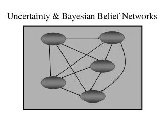
Uncertainty & Bayesian Belief Networks. Data-Mining with Bayesian Networks on the Internet. Internet can be seen as a massive repository of Data Data is often updated Once meaningful data has been collected from the Internet, some model is needed which is able to:

E N D
Data-Mining with Bayesian Networks on the Internet • Internet can be seen as a massive repository of Data • Data is often updated • Once meaningful data has been collected from the Internet, some model is needed which is able to: • be learnt from the vast amount of available data • enable the user to reason about the data. • Be easily updated given new data
Section 1 - Bayesian NetworksAn Introduction • Brief Summary of Expert Systems • Causal Reasoning • Probability Theory • Bayesian Networks - Definition, inference • Current issues in Bayesian Networks • Other Approaches to Uncertainty
1960s - Rule Based Systems Model human Expertise using IF .. THEN rules or Production Rules. Combines the rules (or Knowledge Base) with an inference engine to reason about the world. Given certain observations, produces conclusions. Relatively successful but limited. Expert Systems1 Rule Based Systems
Rule based systems failed to handle uncertainty Only dealt with true or false facts Partly overcome using Certainty factors However, other problems: no differentiation between causal rules and diagnostic rules. 2 Uncertainty
Model Domain rather than Expert Classical probability used rather than ad-hoc calculus Expert support rather than Expert Model 1980s - More Powerful Computers make complex probability calculations feasible Bayesian Networks introduced (Pearl 1986) e.g. MUNIN. 3 Normative Expert Systems
Causality - 1 Icy Roads Icy Roads Holmes Crashes Watson Crashes
- 2 Wet Grass Rain Sprinkler Watson’s Grass Wet Holmes’ Grass Wet
- 3 Earthquake or Burglar Burglary Earthquake Alarm Mary Calls John Calls
All probabilities are between 0 and 1 Necessarily true propositions have probability=1 and necessarily false propositions have probability=0 Tour through Probability
Conjunctions and Disjunctions Venn Diagrams • P(A & B) = P(A) x P(B) • P(A v B) = P(A) + P(B) (mutually exclusive) • P(A v B) =P(A)+P(B) - P(A & B) (not mutually exclusive) A B A B A B
Conditional probability & independence • Probability of B “given” A: • Independence: P(B|A)=P(A&B) P(A) E.g. P(Hearts|Heart last time) P(B|A)=P(B) E.g. P(Heads|Even) = P(Heads)
Probability Distributions • Probability Distribution: • p(Weather=Sunny) = 0.5 • p(Weather=Rain)= 0.2 • p(Weather=Cloud)= 0.2 • p(Weather=Snow)= 0.1 • NB Distribution sums to 1. 0.5 0.2 0.1 S R C S
Completely specifies all beliefs in a problem domain. Joint prob Distribution is an n-dimensional table with a probability in each cell of that state occurring. Written as P(X1, X2, X3 …, Xn) When instantiated as P(x1,x2 …, xn) Joint Probability
Joint Distribution Example • Domain with 2 variables each of which can take on 2 states. P(Toothache, Cavity) Toothache ¬Toothache Cavity 0.04 0.06 ¬Cavity 0.01 0.89
Bayes’ Theorem Simple: P(Y|X) = P(X|Y)P(Y) P(X) General: P(Y|X,E) = P(X|Y,E)P(Y|E) P(X|E)
Bayesian Probability • No need for repeated Trials • Appear to follow rules of Classical Probability • How well do we assign probabilities? The Probability Wheel: A Tool for Assessing Probabilities
Bayesian Network - Definition • Causal Structure • Interconnected Nodes • Directed Acyclic Links • Joint Distribution formed from conditional distributions at each node.
Earthquake or Burglar Burglary Earthquake Alarm Mary Calls John Calls
Bayesian Network for Alarm Domain Burglary Earthquake P(B) P(E) .001 .002 B E P(A) T T .95 T F .94 Alarm F T .29 F F .001 A P(M) A P(J) T .70 T .90 F .01 F .05 Mary Calls John Calls
Retrieving Probabilities from the Conditional Distributions n • P(x1,…xn) = PP(xi|Parents(xi)) • E.g. P(J & M & A & ¬B & ¬E) = P(J|A)P(M|A)P(A|¬B,¬E)P(¬B)P(¬E) = 0.9 x 0.7 x 0.001 x 0.999 x 0.998 = 0.00062 i=1
Constructing A Network- Node Ordering and Compactness • Mary Calls • John Calls • Alarm • Burglary • Earthquake Mary Calls John Calls Alarm Burglary Earthquake
Node Ordering and Compactness contd. • Mary Calls • Johns Calls • Earthquake • Burglary • Alarm
Node Ordering and Compactness contd. • Mary Calls • Johns Calls • Earthquake • Burglary • Alarm Mary Calls John Calls Earthquake Burglary Alarm
Conditional Independence revisited - D-Separation • To do inference in a Belief Network we have to know if two sets of variables are conditionally independent given a set of evidence. • Method to do this is called Direction-Dependent Separation or D-Separation.
D-Separation contd. • If every undirected path from a node in X to a node in Y is d-separated by E, then X and Y are conditionally independent given E. • X is a set of variables with unknown values • Y is a set of variables with unknown values • E is a set of variables with known values.
D-Separation contd. • A set of nodes, E, d-separates two sets of nodes, X and Y, if every undirected path from a node in X to a node in Y is Blocked given E. • A path is blocked given a set of nodes, E if: 1) Z is in E and Z has one arrow leading in and one leading out. 2) Z is in E and has both arrows leading out. 3) Neither Z nor any descendant of Z is in E and both path arrows lead in to Z.
Blocking X Y E Z Z Z
D-Separation - Example Battery • Moves and Battery are independent given it is known about Ignition • Moves and Radio are independent if it is known that Battery works • Petrol and Radio are independent given no evidence. But are dependent given evidence of Starts Radio Ignition Petrol Starts Moves
Inference • Diagnostic Inferences (effects to causes) • Causal Inferences (causes to effects) • Intercausal Inferences - or ‘Explaining Away’ (between causes of common effect) • Mixed Inferences (combination of two or more of the above)
Inference contd. Q E Q E E Q E Q E Diagnostic Causal Intercausal Mixed
Inference contd. Burglary Earthquake Alarm Mary Calls John Calls
Inference in Singly Connected Networks • E.g. P(X|E): Involves computing two values: • Causal Support (evidence variables above X connected through it’s parents) • Evidential Support (evidence variables below X connected through it’s children • Algorithm can perform in Linear Time.
Inference Algorithm E Spreads out from Q to evidence nodes, root nodes and leaf nodes. Each recursive call excludes the node from which it was called. Causal Support Q E E Evidential Support
Inference in Multiply Connected Networks • Exact Inference is known to be NP-Hard • Approaches include: • Clustering • Conditioning • Stochastic Simulation • Stochastic Simulation is most often used, particularly on large networks.
Clustering Cloudy Cloudy Sprinkler Rain Sprinkler & Rain P(S&R) C P(R) T .08 .02 F .40 .10 C TT TF FT FF T .08 .02 .72 .18 F .40 .10 .40 .10 C P(S) T .08 .02 F .40 .10 Wet Grass Wet Grass
Conditioning - - + + Cloudy Cloudy Cloudy Cloudy Sprinkler Rain Sprinkler Rain Wet Grass Wet Grass
Stochastic Simulation - Example P(A=1) = 0.2 A A P(B=1) 0 0.2 1 0.8 A p(C=1) 0 0.05 1 0.2 B C E D
StochasticSimulationRun repeated simulations to estimate the probability distribution • Let Wx = the states of all other variables except x. • Let the Markov Blanket of a node be all of its parents, children and parents of children. • Distribution of each node, x, conditioned upon Wx can be computed locally from their own probability with their children’s : • P(a|Wa) = . P(a) . P(b|a) . P(c|a) • P(b|Wb) = . P(b|a) . P(d|b,c) • P(c|Wc) = . P(c|a) . P(d|b,c) . P(e|c) • Therefore, only the Markov blanket of a node is required to compute the distribution
The Algorithm • Set all observed nodes to their values • Set all other nodes to random values • STEP 1 • Select a node randomly from the network • According to the states of the node’s markov blanket, compute P(x=state, Wx) for all states • STEP 2 • Use a random number generator that is biased according to the distribution computed in step 1 to select the next value of the node • Repeat
Algorithm contd. • The final probability distribution of each unobserved node is calculated from either: 1) the number of times each node took a particular state 2) the average conditional probability of each node taking a particular state given the other variables states.
Case Study - Pathfinder • Diagnostic Expert System for Lymph-Node Diseases 4 Versions of Pathfinder : 1) Rule Based 2) Experimented with Certainty Factors/Dempster-Shafer theory/Bayesian Models 3) Refined Probabilities 4) Refined dependencies
Section 2 - Research Issues in Uncertainty 1 Learning Belief Networks from Data • Assume no Knowledge of Probabilities Distributions or Causal Structure. • Is it possible to infer both of these from data? Case Fraud Gas Jewellery Age Sex 1 No No No 30-50 F 2 No No No 30-50 M 3 Yes Yes Yes >50 M 4 No No No 30-50 M 5 No Yes No <30 F 6 No No No <30 F 7 No No No >50 M 8 No No Yes 30-50 F 9 No Yes No <30 M 10 No No No <30 F
Some Methods • Bayesian (Cooper & Herskovitz 1991) • Minimum Description Length (Lam & Bachus 1994) • Bound and Collapse (Ramoni 1996) Fraud Age Sex Gas Jewelry
2 Dynamics - Markov Models State Transition Model State t-2 State t-1 State t State t+1 State t+2 Percept t-2 Percept t-1 Percept t Percept t+1 Percept t+2 Sensor Model
Updating over time State t-1 State t Percept t-1 Percept t State t Percept t State t State t+1 Percept t Percept t+1
Dynamic Belief Networks - Forecasting Car sales t-1 t Price Price Demand Health Demand Health Supply Supply
3 Other approaches to modeling Uncertainty • Default Reasoning • Dempster - Shafer Theory • Fuzzy Logic ?