Download
1 / 15
170 likes | 438 Views
Controller Tuning Relations. In the last section, we have seen that model-based design methods such as DS and IMC produce PI or PID controllers for certain classes of process models. IMC Tuning Relations.

E N D
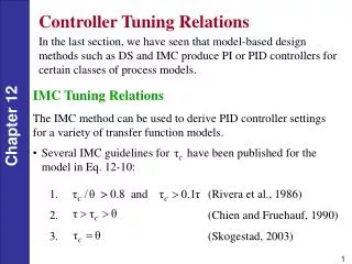
Controller Tuning Relations In the last section, we have seen that model-based design methods such as DS and IMC produce PI or PID controllers for certain classes of process models. IMC Tuning Relations The IMC method can be used to derive PID controller settings for a variety of transfer function models. • Several IMC guidelines for have been published for the model in Eq. 12-10: • > 0.8 and (Rivera et al., 1986) • (Chien and Fruehauf, 1990) • (Skogestad, 2003)
Table 12.1 IMC-Based PID Controller Settings for Gc(s) (Chien and Fruehauf, 1990). See the text for the rest of this table.
Tuning for Lag-Dominant Models • First- or second-order models with relatively small time delays are referred to as lag-dominant models. • The IMC and DS methods provide satisfactory set-point responses, but very slow disturbance responses, because the value of is very large. • Fortunately, this problem can be solved in three different ways. • Method 1: Integrator Approximation • Then can use the IMC tuning rules (Rule M or N) to specify the controller settings.
Method 2. Limit the Value of tI • For lag-dominant models, the standard IMC controllers for first-order and second-order models provide sluggish disturbance responses because is very large. • For example, controller G in Table 12.1 has where is very large. • As a remedy, Skogestad (2003) has proposed limiting the value of : where t1 is the largest time constant (if there are two). Method 3. Design the Controller for Disturbances, Rather Set-point Changes • The desired CLTF is expressed in terms of (Y/D)des, rather than (Y/Ysp)des • Reference: Chen & Seborg (2002)
Example 12.4 Consider a lag-dominant model with Design four PI controllers: • IMC • IMC based on the integrator approximation • IMC with Skogestad’s modification (Eq. 12-34) • Direct Synthesis method for disturbance rejection (Chen and Seborg, 2002): The controller settings are Kc = 0.551 and
Evaluate the four controllers by comparing their performance for unit step changes in both set point and disturbance. Assume that the model is perfect and that Gd(s) = G(s). Solution The PI controller settings are:
Figure 12.8. Comparison of set-point responses (top) and disturbance responses (bottom) for Example 12.4. The responses for the Chen and Seborg and integrator approximation methods are essentially identical.
Tuning Relations Based on Integral Error Criteria • Controller tuning relations have been developed that optimize the closed-loop response for a simple process model and a specified disturbance or set-point change. • The optimum settings minimize an integral error criterion. • Three popular integral error criteria are: • Integral of the absolute value of the error (IAE) where the error signal e(t) is the difference between the set point and the measurement.
Figure 12.9. Graphical interpretation of IAE. The shaded area is the IAE value. Chapter 12a
Integral of the squared error (ISE) • Integral of the time-weighted absolute error (ITAE) See text for ITAE controller tuning relations.
Comparison of Controller Design and Tuning Relations Although the design and tuning relations of the previous sections are based on different performance criteria, several general conclusions can be drawn:
The controller gain Kc should be inversely proportional to the product of the other gains in the feedback loop (i.e., Kc 1/K where K = KvKpKm). • Kc should decrease as , the ratio of the time delay to the dominant time constant, increases. In general, the quality of control decreases as increases owing to longer settling times and larger maximum deviations from the set point. • Both and should increase as increases. For many controller tuning relations, the ratio, , is between 0.1 and 0.3. As a rule of thumb, use = 0.25 as a first guess. • When integral control action is added to a proportional-only controller, Kc should be reduced. The further addition of derivative action allows Kc to be increased to a value greater than that for proportional-only control.