Download
1 / 33
330 likes | 354 Views
This book explores the algorithms and applications of PDE-constrained optimization in computational science and engineering, covering topics such as forward and inverse problems, Karush-Kuhn-Tucker conditions, global optimization, and more. It discusses challenges and solutions for large-scale problems and provides illustrations of PDE-based optimization in various fields.

E N D
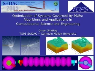
Optimization of Systems Governed by PDEs: Algorithms and Applications in Computational Science and EngineeringOmar GhattasTOPS SciDAC + Carnegie Mellon University
Given est. of d, solve state eqn for u Given d& u, solve adjoint eqn for p Given u& p, solve opt eqn to update d A peak at the basic algorithm Numerous issues related to globalization, inexactness, time dependent problems, continuation, preconditioning, Krylov solvers, multilevel algorithms See V. Akcelik, G. Biros, O. Ghattas, J. Hill, D. Keyes, and B. van Bloemen Waanders, “Parallel Algorithms for PDE-constrained optimization”, Frontiers of Parallel Scientific Computing, M. Heroux, P. Raghavan, and H. Simon, eds., SIAM, 2006, to appear.
PDE-constrained optimization: Why now? • Maturing state of models, discretization, and solvers for forward problems • Emergence of large-scale finite-dimensional nonlinear optimization algorithms • Rapid rise in high-end computing capability • Improvements in quality of observational data • Optimization is often what is of ultimate interest
PDE-constrained optimization: Challenges • All of the forward simulation components must be automated, online, and parallel • For large optimization variable dimensions (or for high precision), need gradient (and often Hessian) based algorithms • Efficient gradients require adjoint PDE solves • Specialized algorithms required for solution of the coupled optimality system • Optimization of terascale-class problems is a petascale-level challenge
Illustrations of PDE-based optimization • Optimal control: • Optimal boundary control of Navier-Stokes flows (*) • Inverse problems: • Earthquake inversion for earth properties (*) • Optimal design: • Shape optimization of linear accelerators * = PETSc-powered
Optimal boundary flow control minimize subject to: Joint work with George Biros, Penn [SIAM J Sci Comp 2005]
Strong form of 1st order optimality system • Forward problem • Adjoint • Control
Flow around Boeing 707 Wing • 700,000 states • 4,000 controls • 128 procs (T3E) • ~5 hrs (LNKS-PR-TN) • Continuation
Flow around Boeing 707 Wing Uncontrolled Controlled
Volkan Akcelik, Aysegul Askan, Jacobo Bielak, George Biros (Penn), Omar Ghattas, Kwan-Liu Ma (UC-Davis), David O’Hallaron, Leonardo Ramirez, Tiankai Tu, Hongfeng Yu (UC-Davis) Earthquake modeling for seismic hazard assessment Region of interest for 1994 Northridge earthquake simulation Adaptive grid resolves up to 1Hz freq. w/100 million grid pts; uniform grid would require 2000x more points SCEC geological model provides 3D soil properties in Greater LA Basin Inversion of surface observations for 17 million elastic parameters (right: target; left: inversion result) Comparison of observation with simulation (improved prediction requires petaflops capability) Snapshot of simulated ground motion (simulation requires 3hr on 6Tflops PSC machine, running at >80% parallel eff)
Forward earthquake modeling Variable-slip kinematic source model USGS
Target vs. inverted isosurfaces(Gordon Bell Prize @ SC2003) 17M inversion parameters, 70B total variables, 24 hours on 2048 processors of AlphaCluster at PSC
Comparison of target and inverted material models: 3D acoustic and elastic Acoustic medium, p-wave velocity Elastic medium, s-wave velocity
Shape Optimization for Accelerator Structures Patrick Knupp Tim Tautges Lori Diachin Mark Shephard Rich Lee Kwok Ko Volkan Akcelik Omar Ghattas George Biros David Keyes Esmond Ng
Basic Analysis Loop for given Geometry p-refinement h-Refinement Omega3P S3P T3P Tau3P Refinement Partitioning (parallel) Solvers (parallel) CAD Meshing Shape Optimization for Accelerator Structures • Numerical modeling has replaced trial and error prototyping approach • SciDAC adds advances that increase fidelity, speed, and accuracy: DDS CELL • Next generation accelerators have complex cavities that require shape optimization for improved performance and reduced cost • AST/TOPS/TSTT are collaborating to develop an automated capability to accelerate this otherwise manual process
Difficulties in Automated Shape Optimization for Accelerator Structures • Gradient-based optimization essential to manage large design space, expensive state simulation (a Maxwell eigenvalue solve for frequencies of interest), and high accuracy requirements • Need to compute derivatives of design goals with respect to design parameters (CAD parameterization of geometry • Finite difference approximation of gradient inaccurate and intractable: would require tens of eigenvalue solves per design iteration! • Optimization of shape often requires derivatives of mesh motion and CAD parameterization • Remeshing new geometry necessary at each design iteration • All function and gradient computations, remeshing, and optimization steps must scale well to large numbers of state parameters and processors
Approach for Addressing Difficulties • Adopt adjoint sensitivity methods: only a handful of (linearized) eigenvalue solves needed at each design iteration (but need to develop capability to solve adjoint eigenvalue problem) • Compute gradient from infinite-dimensional form: avoids differentiation of meshing algorithm (but need to develop capability to evaluate surface integrals with higher-order derivatives of solution and geometry) • Build on TSTT parallel remeshing and CAD capabilities • Tailor TOPS parallel optimization algorithms to structure of accelerator design problem
Component Interoperation forShape Optimization with Omega3P Solver geometric model Omega3P Sensitivity optimization meshing sensitivity Omega3P meshing (only for discrete sensitivity)
ILC low loss cavity: 9 cells + 3 coax couplers Goal: damp trapped mode(s) while maintaining accelerating frequency of 1.3 Ghz Means: optimize shape of end cell
Shape optimization problem: Damp well-trapped dipole modes while maintaining the accelerating frequency
Optimality conditions (consider one controlled mode, penalize frequency)
5 2 3 6 c 4 b 1 a Comparison of Sensitivity for 1/Q c=0.10 a=0.08 b=0.06
c b a Minimizing 1/Q with Freq=2.0GHz Electric BC on all surfaces
Optimizing ILC-like Cavity • ILC-like cavity with 9-cells: 7 mid-cells are identical and fixed, while the shapes of the two end cells are to be optimized • Analytical formula for design velocity (derivatives of surface points w.r.t. design variables) • Analytical formula for mesh movement
End Cell Dimensions • The cell is cylindrically symmetric and consists of 4 quarters of ellipse curves (ai, bi) • We choose R, a1, b1, and b as independent design variables • Others are either dependent (a2,b2,…) or fixed (L, a4, b4, …) a1 b2 b1 a2 R L b
ILC-like shape optimization: first results • Maximize the stored energy of a dipole mode in the end cell while satisfying acc - * = 0 • Initial design variables: • R=41mm,a1=17.590mm, b1=20mm,b=103.36mm • Uendcell = 0.31%, = -0.04756 • After five optimization iterations, optimized solution is found: • R=40.992mm, a1=17.571mm b1=20.008mm, b=103.455mm • Uendcell = 0.49%, = -3.75e-6
Final Remarks • Maturing state of forward solvers and emerging capabilities for PDE-constrained optimization invite what is often the ultimate goal: simulation-based optimization (design, control, inversion) • Optimization problems with 106 – 108 variables can be solved in as little as 5-10X the forward simulation time • Shape optimization brings additional challeges of the highest order: • requires CAD/mesh/solvers to be fast, automated, differentiable, scalable • Continuous adjoints provide design variable independence, require only surface mesh sensititivies • Parallel mesh movement capability essential • Huge effort: worse than writing solver code from scratch • But huge potential payoff for design of multi-billion dollar devices