Fin500J: Mathematical Foundations in Finance Topic 6: Ordinary Differential Equations

1. Fin500J: Mathematical Foundations in Finance Topic 6: Ordinary Differential Equations Philip H. Dybvig Reference: Lecture Notes by Paul Dawkins, 2007, page 20-33, page 102-121, page 137-155 and page 340-344 http://tutorial.math.lamar.edu/terms.aspx Slides designed by Yajun Wang Fall 2010 Olin Business School

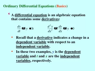
2. Introduction to Ordinary Differential Equations (ODE) • Recall basic definitions of ODE, • order • linearity • initial conditions • solution • Classify ODE based on( order, linearity, conditions) • Classify the solution methods Fall 2010 Olin Business School

3. Derivatives Derivatives Ordinary Derivatives y is a function of one independent variable Partial Derivatives u is a function of more than one independent variable Fall 2010 Olin Business School

4. Differential Equations Differential Equations Ordinary Differential Equations involve one or more Ordinary derivatives of unknown functions involve one or more partial derivatives of unknown functions Partial Differential Equations Fall 2010 Olin Business School

5. Ordinary Differential Equations Ordinary Differential Equations (ODE) involve one or more ordinary derivatives of unknown functions with respect to one independent variable y(x): unknown function x: independent variable Fall 2010 Olin Business School

6. Order of a differential equation The order of an ordinary differential equations is the order of the highest order derivative First order ODE Second order ODE Second order ODE Fall 2010 Olin Business School

7. Solution of a differential equation A solution to a differential equation is a function that satisfies the equation. Fall 2010 Olin Business School

8. Linear ODE An ODE is linear if the unknown function and its derivatives appear to power one. No product of the unknown function and/or its derivatives Linear ODE Linear ODE Non-linear ODE Fall 2010 Olin Business School

9. same different Boundary-Value and Initial value Problems Boundary-Value Problems • The auxiliary conditions are not at one point of the independent variable • More difficult to solve than initial value problem Initial-Value Problems • The auxiliary conditions are at one point of the independent variable Fall 2010 Olin Business School

10. Classification of ODE ODE can be classified in different ways • Order • First order ODE • Second order ODE • Nth order ODE • Linearity • Linear ODE • Nonlinear ODE • Auxiliary conditions • Initial value problems • Boundary value problems Fall 2010 Olin Business School

11. Solutions • Analytical Solutions to ODE are available for linear ODE and special classes of nonlinear differential equations. • Numerical method are used to obtain a graph or a table of the unknown function • We focus on solving first order linear ODE and second order linear ODE and Euler equation Fall 2010 Olin Business School

12. First Order Linear Differential Equations • Def: A first order differential equation is said to be linear if it can be written Fall 2010 Olin Business School

13. First Order Linear Differential Equations • How to solve first-order linear ODE ? Sol: Multiplying both sides by , called an integrating factor, gives assuming we get Fall 2010 Olin Business School

14. First Order Linear Differential Equations By product rule, (4) becomes Now, we need to solve from (3) Fall 2010 Olin Business School

15. First Order Linear Differential Equations to get rid of one constant, we can use Fall 2010 Olin Business School

16. Summary of the Solution Process • Put the differential equation in the form (1) • Find the integrating factor, using (8) • Multiply both sides of (1) by and write the left side of (1) as • Integrate both sides • Solve for the solution Fall 2010 Olin Business School

17. Example 1 Sol: Fall 2010 Olin Business School

18. Example 2 Sol: Fall 2010 Olin Business School

19. Second Order Linear Differential Equations • Homogeneous Second Order Linear Differential Equations • real roots, complex roots and repeated roots • Non-homogeneous Second Order Linear Differential Equations • Undetermined Coefficients Method • Euler Equations Fall 2010 Olin Business School

20. Second Order Linear Differential Equations The general equation can be expressed in the form where a, b and c are constant coefficients Let the dependent variable y be replaced by the sum of the two new variables: y = u + v Therefore If v is a particular solution of the original differential equation purpose The general solution of the linear differential equation will be the sum of a “complementary function” and a “particular solution”. Fall 2010 Olin Business School

21. The Complementary Function (solution of the homogeneous equation) Let the solution assumed to be: characteristic equation Real, distinct roots Double roots Complex roots Fall 2010 Olin Business School

22. Real, Distinct Roots to Characteristic Equation • Let the roots of the characteristic equation be real, distinct and of values r1 and r2. Therefore, the solutions of the characteristic equation are: • The general solution will be • Example Fall 2010 Olin Business School

23. Equal Roots to Characteristic Equation • Let the roots of the characteristic equation equal and of value r1 = r2 = r. Therefore, the solution of the characteristic equation is: Let where V is a function of x Fall 2010 Olin Business School

24. Complex Roots to Characteristic Equation Let the roots of the characteristic equation be complex in the form r1,2 =λ±µi. Therefore, the solution of the characteristic equation is: Fall 2010 Olin Business School

25. Examples (I) Solve (II) Solve characteristic equation characteristic equation Fall 2010 Olin Business School

26. Non-homogeneous Differential Equations (Method of Undetermined Coefficients) When g(x) is constant, say k, a particular solution of equation is When g(x) is a polynomial of the form where all the coefficients are constants. The form of a particular solution is Fall 2010 Olin Business School

27. Example Solve complementary function characteristicequation equating coefficients of equal powers of x Fall 2010 Olin Business School

28. Non-homogeneous Differential Equations (Method of Undetermined Coefficients) • When g(x) is of the form Terx, where T and r are constants. The • form of a particular solution is • When g(x) is of the form Csinnx + Dcosnx, where C and D are • constants, the form of a particular solution is Fall 2010 Olin Business School

29. Example complementary function Solve characteristic equation Fall 2010 Olin Business School

30. Example complementary function Solve characteristic equation Fall 2010 Olin Business School

31. Example complementary function Solve characteristic equation Fall 2010 Olin Business School

32. Euler Equations • Def: Euler equations • Assuming x>0 and all solutions are of the form y(x) = xr • Plug into the differential equation to get the characteristic equation Fall 2010 Olin Business School

33. Solving Euler Equations: (Case I) • The characteristic equation has two different real solutions r1 and r2. • In this case the functions y = xr1 and y = xr2 are both solutions to the original equation. The general solution is: Example: Fall 2010 Olin Business School

34. Solving Euler Equations: (Case II) • The characteristic equation has two equal roots r1 = r2=r. • In this case the functions y = xr and y = xr lnx are both solutions to the original equation. The general solution is: Example: Fall 2010 Olin Business School

35. Solving Euler Equations: (Case III) • The characteristic equation has two complex roots r1,2 = λ±µi. Example: Fall 2010 Olin Business School