Ordinary Differential Equations
230 likes | 581 Views
This outline covers solving Ordinary Differential Equations (ODEs) and optimization problems using Matlab. Learn about numerical solutions, Euler and Runge-Kutta methods, Matlab's ODE solvers, and optimization techniques. Explore Matlab syntax, parameters, polymorphic functions, and optimization functions. Get insights on implementing f functions, solving nonlinear ODEs, and optimizing your code efficiently.

Ordinary Differential Equations
E N D
Presentation Transcript
Outline Announcements: Homework II: Solutions on web Homework III: due Wed. by 5, by e-mail Homework II Differential Equations Numerical solution of ODE’s Matlab’s ODE solvers Optimization problems Matlab’s optimization routines
Homework II Emphasis was on writing functions P.2: Only way to get R into ll2xy is through function argument: function [x,y]=ll2xy(lat,lon,ref,R); P.8: Most confusion stems from definition of the running mean. A few others were less clear on programming
Running Mean • Running mean takes the mean of successive data blocks: • Ex: n=3, x is length 6 y x y is m-n+1
Running Mean • for j=1:m-n+1 %loop over length of y • end
RunningMean • Another option: y=zeros(m-n+1,1); for k=1:n y=y+x(k:k+m-n); end y=y/n; • Which is faster, looping over m or n?
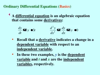
Differential Equations Ordinary differential equations (ODE’s) arise in almost every field ODE’s describe a function y in terms of its derivatives The goal is to solve for y
Example: Logistic Growth N(t) is the function we want (number of animals)
Numerical Solution to ODEs In general, only simple (linear) ODEs can be solved analytically Most interesting ODEs are nonlinear, must solve numerically The idea is to approximate the derivatives by subtraction
Euler Method Simplest ODE scheme, but not very good “1st order, explicit, multi-step solver” General multi-step solvers: (weighted mean of f evaluated at lots of t’s)
Runge-Kutta Methods Multi-step solvers--each N is computed from N at several times can store previous N’s, so only one evaluation of f/iteration Runge-Kutta Methods: multiple evaluations of f/iteration:
Matlab’s ODE solvers Matlab has several ODE solvers: ode23 and ode45 are “standard” RK solvers ode15s and ode23s are specialized for “stiff” problems several others, check help ode23 or book
All solvers use the same syntax: [t,N]=ode23(@odefile, t, N0, {options, params …}) odefile is the name of a function that implements f function f=odefile(t, N, {params}), f is a column vector t is either [start time, end time] or a vector of times where you want N N0= initial conditions options control how solver works (defaults or okay) params= parameters to be passed to odefile Matlab’s ODE solvers
Parameters To accept parameters, your ode function must be polymorphic f=odefile(t,x); f=odefile(t,x,params); function f=odefile(t,x,params); if(nargin<3) params=defaults; end f=…
Matlab functions can be polymorphic--the same function can be called with different numbers and types of arguments Example: plot(y), plot(x,y), plot(x,y,’rp’); In a function, nargin and nargout are the number of inputs provided and outputs requested by the caller. Even more flexibility using vargin and vargout nargin
Example: Lorenz equations Simplified model of convection cells In this case, N is a vector =[x,y,z] and f must return a vector =[x’,y’,z’]
Optimization For a function f(x), we might want to know at what value of x is f smallest largest? equal to some value? All of these are optimization problems Matlab has several functions to perform optimization
Optimization Simplest functions are x=fzero(@fun, x0);%Finds f(x)==0 starting from x0 x=fminbnd(@fun, [xL, xR]); %Finds minimum in interval [xL,xR] x=fminsearch(@fun,x0); %Finds minimum starting at x0 All of these functions require you to write a function implementing f: function f=fun(x);%computes f(x)
Optimization Toolbox More optimization techniques, but used in the same way Some of these functions can make use of gradient information in higher dimensions, gradient tells you which way to go, can speed up procedure f df/dx = 0
Optimization Toolbox To return gradient information, your function must be polymorphic: x=fun(x) %return value [x,dx]=fun(x); %return value and gradient function [x,dx]=fun(x); if(nargout>1) dx=… end x=…