
Exploring MaxEnt for Species Distribution Modeling
E N D
Presentation Transcript
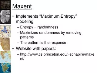
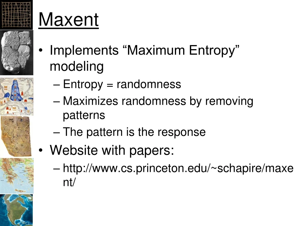
Maxent • Implements “Maximum Entropy” modeling • Entropy = randomness • Maximizes randomness by removing patterns • The pattern is the response • Website with papers: • http://www.cs.princeton.edu/~schapire/maxent/
Overall Definitions • Overall area used to create the model: • Sample area, area-of-interest (AOI), background • Locations where species was observed: • Occurrences, presence points, observations • Environmental predictors: • Covariates, independent variables • Probability density function: • A function showing the probably of values for a covariate • Area under the function must equal 1
Definitions • = sample area (bounds of raster data) • = vector of covariates (e.g. rasters) • = probability density function of the covariates • Histogram of covariates divided by (number of pixels in sample area) • = locations of occurrences (pixels in covariates where occurrences exist) • = probability density function of the covariates where there are occurrences • Histogram of covariates where there are occurrences divided by (number of pixels with occurrences)
Relationships of histograms to probability distributions N Histogram of all covariate values Histogram of covariate values at occurrences Frequency 0 Min Covariate (precip, temp, aspect, distance from…) Max
Densities • = Maxent’s raw output 1 Highest density of occurrences (best habitat) No occurrences (not habitat) 0 Min Covariate (precip, temp, aspect, distance from…) Max
Densities From Elith et. al.
MaxEnt’s “Model” • The Model: • Where • normalizing constant • vector of coeficients • = vector of “Features” • The “target” of MaxEnt is: • This is a log-linear model similar to GLMs • (but the model can be much more complex)
MaxEnt Optimizes “Gain” • “Gain in MaxEnt is related to deviance” • See Phillips in the tutorial • MaxEnt generates a probability distribution of pixels in the grid starting at uniform and improving the fit to the data • “Gain indicates how closely the model is concentrated around presence samples” • Phillips
Gain • Gain is the average log probability of each point. • : makes gain=0 for uniform • Gain is the average log-likelihood minus C
Regularization • Regularization for each coefficient • :penalty for over fitting • MaxEnt Maximizes: • In other words: • Tries to have the highest likelihood • And • The smallest number of coefficients • The Regularization Parameter increases the penalty for coefficients • Related to AIC
Background Points • 10,000 random points (default) • Uses all pixels if <10,000 samples
MaxEnt really… • MaxEnt tries to create a probability surface in hyperspace where: • Values are near 1.0 where there are lots of points • Values are near 0.0 where there are few or no points
Threshold~0.5 Threshold~0.2 Threshold~0.0
Cumulative Threshold All points omitted for no area Threshold of 0 = Entire area Threshold of 100% = no area No omission for entire area
Definitions • Omission Rate: Proportion of points left out of the predicted area for a threshold • Sensitivity: Proportion of points left in the predicted area • 1 – Omission Rate • Fractional Predicted Area: • Proportion of area within the thresholded area • Specificity: Proportion of area outside the thresholded area • 1 – Fractional Predicted Area:
Receiver-Operator Curve (ROC) Area Under The Curve (AUC)
What proportion of the sample points are within the thresholded area Goes up quickly if points are within a sub-set of the overall predictor values What proportion of the total area is within the thresholded area
AUC Area Under the Curve 0.5=Model is random, Closer to 1.0 the better
Best Explanation Ever! http://en.wikipedia.org/wiki/Receiver_operating_characteristic
Fitting Features • Types of “Features” • Threshold: flat response to predictor • Hinge: linear response to predictor • Linear: linear response to predictor • Quadratic: square of the predictor • Product: two predictors multiplied together • Binary: Categorical levels • The following slides are from the tutorial you’ll run in lab
Getting the “Best” Model • AUC does not account for the number of parameters • Use the regularization parameter to control over-fitting • MaxEnt will let you know which predictors are explaining the most variance • Use this, and your judgment to reduce the predictors to the minimum number • Then, rerun MaxEnt for final outputs
Number of Parameters cld6190_ann, 0.0, 32.0, 84.0 dtr6190_ann, 0.0, 49.0, 178.0 ecoreg, 0.0, 1.0, 14.0 frs6190_ann, -1.1498818281061252, 0.0, 235.0 h_dem, 0.0, 0.0, 5610.0 pre6190_ann, 0.0, 0.0, 204.0 pre6190_l1, 0.0, 0.0, 185.0 pre6190_l10, 0.0, 0.0, 250.0 pre6190_l4, 0.0, 0.0, 188.0 pre6190_l7, 0.0, 0.0, 222.0 tmn6190_ann, 0.0, -110.0, 229.0 tmp6190_ann, 0.5804254993432195, 1.0, 282.0 tmx6190_ann, 0.0, 101.0, 362.0 vap6190_ann, 0.0, 1.0, 310.0 tmn6190_ann^2, 1.0673168197973097, 0.0, 52441.0 tmx6190_ann^2, -4.158022614271723, 10201.0, 131044.0 vap6190_ann^2, 0.8651171091826158, 1.0, 96100.0 cld6190_ann*dtr6190_ann, 1.2508669203612586, 2624.0, 12792.0 cld6190_ann*pre6190_l7, -1.174755465148628, 0.0, 16884.0 cld6190_ann*tmx6190_ann, -0.4321445358008761, 3888.0, 28126.0 cld6190_ann*vap6190_ann, -0.18405049411034943, 38.0, 25398.0 dtr6190_ann*pre6190_l1, 1.1453859981618322, 0.0, 19240.0 dtr6190_ann*pre6190_l4, 4.849148645354156, 0.0, 18590.0 dtr6190_ann*tmn6190_ann, 3.794041694656147, -16789.0, 23843.0 ecoreg*tmn6190_ann, 0.45809862608857377, -1320.0, 2290.0 ecoreg*tmx6190_ann, -1.6157434815320328, 154.0, 3828.0 ecoreg*vap6190_ann, 0.34457033151188204, 12.0, 3100.0 frs6190_ann*pre6190_l4, 2.032039282175344, 0.0, 6278.0 frs6190_ann*tmp6190_ann, -0.7801709867413774, 0.0, 15862.0 frs6190_ann*vap6190_ann, -3.5437330369989097, 0.0, 11286.0 h_dem*pre6190_l10, 0.6831004745857797, 0.0, 332920.0 h_dem*pre6190_l4, -7.446077252168424, 0.0, 318591.0 pre6190_ann*pre6190_l7, 1.5383313604986337, 0.0, 39780.0 pre6190_l1*vap6190_ann, -2.6305122968909807, 0.0, 47495.0 pre6190_l10*pre6190_l4, -2.5355630131828004, 0.0, 47000.0 pre6190_l10*pre6190_l7, 5.413839860312993, 0.0, 48750.0 pre6190_l10*tmn6190_ann, 1.2055688090972252, -1407.0, 54500.0 pre6190_l4*pre6190_l7, -3.172491547290633, 0.0, 36660.0 pre6190_l4*tmn6190_ann, -1.2333164353879962, -1463.0, 40984.0 pre6190_l4*vap6190_ann, -0.6865648521426311, 0.0, 55648.0 pre6190_l7*tmp6190_ann, -0.45424195658031474, 0.0, 55278.0 pre6190_l7*tmx6190_ann, -0.23195173539212843, 0.0, 68598.0 tmn6190_ann*tmp6190_ann, 0.733594398523686, -6300.0, 64014.0 tmn6190_ann*vap6190_ann, 1.414888294903485, -3675.0, 70074.0 (85.5<pre6190_l10), 0.7526049605127942, 0.0, 1.0 (22.5<pre6190_l7), 0.09143627960137418, 0.0, 1.0 (14.5<pre6190_l7), 0.3540139414522918, 0.0, 1.0 (101.5<tmn6190_ann), 0.5021949716276776, 0.0, 1.0 (195.5<h_dem), -0.4332023993069761, 0.0, 1.0 (340.5<tmx6190_ann), -1.4547597256316012, 0.0, 1.0 (48.5<h_dem), -0.1182394373335682, 0.0, 1.0 (14.5<pre6190_l10), 1.4894000152716946, 0.0, 1.0 (308.5<tmx6190_ann), -0.5743766711031515, 0.0, 1.0 (311.5<tmx6190_ann), -0.19418359220467488, 0.0, 1.0 (23.5<pre6190_l4), 0.6810910505907158, 0.0, 1.0 (9.5<ecoreg), 0.7192087537708799, 0.0, 1.0 (281.5<tmx6190_ann), -1.2177451449751997, 0.0, 1.0 (50.5<h_dem), -0.2041650979073212, 0.0, 1.0 'tmn6190_ann, 2.506694714713521, 228.5, 229.0 (36.5<h_dem), -0.04215558381842702, 0.0, 1.0 (191.5<tmp6190_ann), 0.8679225073207016, 0.0, 1.0 (101.5<dtr6190_ann), 0.0032675586724019226, 0.0, 1.0 'cld6190_ann, -0.009785185080653264, 82.5, 84.0 `h_dem, -1.0415514779720143, 0.0, 2.5 (1367.0<h_dem), -0.2128591450282928, 0.0, 1.0 (280.5<tmx6190_ann), -0.06975266984609022, 0.0, 1.0 (55.5<pre6190_ann), -0.3681568888568664, 0.0, 1.0 (211.5<h_dem), -0.09946657794871552, 0.0, 1.0 (82.5<pre6190_l10), 0.09831192008677023, 0.0, 1.0 (41.5<pre6190_l7), -0.07282871533190113, 0.0, 1.0 (86.5<pre6190_l1), -0.06404898712746389, 0.0, 1.0 (106.5<pre6190_l1), 0.9347973610811197, 0.0, 1.0 (97.5<pre6190_l4), 0.02588993095745272, 0.0, 1.0 `h_dem, 0.2975112175166992, 0.0, 57.5 `pre6190_l1, -1.4918629714740488, 0.0, 3.5 (87.5<pre6190_l1), -0.16210452683985327, 0.0, 1.0 `pre6190_l1, 0.6469706380585183, 0.0, 33.5 (199.5<vap6190_ann), 0.07974469741688692, 0.0, 1.0 `pre6190_l7, 0.6529517367541156, 0.0, 0.5 (985.0<h_dem), 0.5311126727361561, 0.0, 1.0 (12.5<pre6190_l7), 0.15147093558026073, 0.0, 1.0 'dtr6190_ann, 1.9102989446786593, 100.5, 178.0 (24.5<pre6190_l7), 0.22066203658397954, 0.0, 1.0 `h_dem, 0.19290062857835738, 0.0, 58.5 (95.5<pre6190_l4), 0.11847374533530691, 0.0, 1.0 (42.5<pre6190_l10), -0.22634502760604264, 0.0, 1.0 (59.5<cld6190_ann), -0.08833902526182105, 0.0, 1.0 (156.5<tmn6190_ann), -0.3949178282642713, 0.0, 1.0 'vap6190_ann, -0.09749601885757717, 284.5, 310.0 (195.5<pre6190_l10), -0.7064287716566797, 0.0, 1.0 'pre6190_ann, -0.13355287707153143, 198.5, 204.0 (85.5<pre6190_ann), -0.08639349917230135, 0.0, 1.0 `cld6190_ann, -0.8869579099922708, 32.0, 56.5 (127.5<pre6190_l7), 0.16433984792079512, 0.0, 1.0 (310.5<tmx6190_ann), -0.12187855649464616, 0.0, 1.0 (123.5<dtr6190_ann), -0.3879778631592106, 0.0, 1.0 (58.5<cld6190_ann), -0.045757294470318455, 0.0, 1.0 `h_dem, -0.03506780995851361, 0.0, 15.5 `dtr6190_ann, 0.8788733700181052, 49.0, 89.5 (34.5<pre6190_ann), -0.11675983810645604, 0.0, 1.0 `h_dem, -0.07042193156800028, 0.0, 16.5 (195.5<tmp6190_ann), -0.06201919461360444, 0.0, 1.0 linearPredictorNormalizer, 8.791343644655978 densityNormalizer, 129.41735442727088 numBackgroundPoints, 10112 entropy, 7.845994051976282
Running Maxent • Folder for layers: • Must be in ASCII Grid “.asc” format • CSV file for samples: • Must be: Species, X, Y • Folder for outputs: • Maxent will put a number of files here
Avoiding Problems • Create a folder for each modeling exercise. • Add a sub-folder for “Layers” • Layers must have the same extent & number of rows and columns of pixels • Save your samples to a CSV file: • Species, X, Y as columns • Add a sub-folder for each “Output”. • Number or rename for each run • Some points may be missing environmental data
Running Maxent • Batch file: • maxent.bat contents: • java -mx512m -jar maxent.jar • The 512 sets the maximum RAM for Java to use • Double-click on jar file • Works, with default memory
Response Curves Each response if all predictors are used Each response if only one predictor is used
Surface Output Formats • Logistic – 0 to 1 as probability of presence (most commonly used) • Cumulative – Predicted omission rate • Raw – original
Percent Contribution • Precip. contributes the most
Regularization = 2 • AUC = 0.9
Resampling Occurrences • MaxEnt Uses: • Leave-one-out cross-validation (LOOCV) • Break up data set into N “chucks”, run model leaving out each chunk • Replication: MaxEnt’s term for resampling
Optimizing Your Model • Select the “Sample Area” carefully • Use “Percent Contribution”, Jackknife and correlation stats to determine the set of “best” predictors • Try different regularization parameters to obtain response curves you are comfortable with and reduce the number of parameters (and/or remove features) • Run “replication” to determine how robust the model is to your data
Model Optimization & Selection • Modeling approach • Predictor Selection • Coefficients estimation • Validation: • Against sub-sample of data • Against new dataset • Parameter sensitivity • Uncertainty estimation