More on Maxent
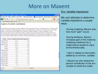
More on Maxent. Env . Variable importance: Ma xent attempts to determine variable importance a couple ways: During modeling, Maxent asks how much “gain” occurs


More on Maxent
E N D
Presentation Transcript
More on Maxent • Env. Variable importance: • Ma xent attempts to determine variable importance a couple ways: • During modeling, Maxent asks how much “gain” occurs • During iterations, Maxent increases gain of the model by modifying coefficient for a single feature based on input environmental data • Gain is related to information added by an environ. variable • Maxent can then determine percent contribution of the env. variable to whole the model
More on Maxent • Env. Variable importance caveats • Percent contribution outputs don’t take into account covariances across environmental layers • Variale importance is based on Maxent algorithm! It might be different using a different method! • Interpret with caution • Permutation importance a new measure.
Env. Variable importance: • Maxent attempts to determine variable importance a couple ways: • jackknifing is another method to determine environmental layer importance • It is a leave-one-layer out without replacement procedure • How much “gain” occurs if we use individual layers or combinations? • Which layer contributes the most gain when used individually?
Env. Variable importance: • comparing test and train variable importance is useful • Note that precip6190_ann is the best predictor for test but not train when used alone • Suggests that transferability of monthly values lower than annual values • Note, length of red bar indicates gain using all variables • If blue bar is shorter than red, corresponding loss of gain (explanation) when variable omitted.
How to read these graphs • Each graph shows the range of values for the pixels in the environment layers you used on the x-axis • Probability of presence is shown on the y-axis (0 to 1) • eg., tmax6190_annshows that for low tmaxs, probability of occurrence is ~1, which drops towards 0 around 22.5 C. • Plots do not take into account correlation among variables • Maxent produces a second graph with individual variables run separately
New Maxent Goodies The Explain Tool • New in Maxent 3.3 • Shows for any point where the value is on all response curves • Can be used to see how env. Variables matter in different areas. • Haven’t had a chance to use this much
How do we know when models are “realistic” or, better put, of “reasonable quality”, or even better put… “valid”?
Two Types of Error in Distributional Predictions Actual geographic distribution
Two Types of Error in Distributional Predictions Predicted geographic distribution
Two Types of Error in Distributional Predictions Actual geographic distribution Predicted geographic distribution
Two Types of Error in Distributional Predictions Actual geographic distribution Predicted geographic distribution Overprediction, or Commission Underprediction, or Omission
Two Types of Error in Distributional Predictions Objective: To Minimize Both Forms of Error
Two Types of Error in Distributional Predictions Objective: To Minimize Both Forms of Error
To evaluate model quality you need to: 1. Generate an ‘independent’ set of data There are at least two strategies to do so:- Collect New Data- Split your data intotwo sets, one set used in training, one set used in modeltesting.
Actually Present Actually Absent Predicted Present a b Predicted Absent c d 3. Quantify error components with a confusion matrix by utilizing the testing data a & d = correct predictionsb = commission error (false positives, overprediction)c = omission error (false negatives, underprediction)
Measuring Omission Redux • Omission error is “easy” to measure if you have a test and training datset • Training dataset to create model • Test dataset to verify if suitable habitats include the “pixels” that also contain the test locations. • If yes, then omission error is low.
Measuring Commission Error Redux • Measuring commission error is much trickier • We don’t know anything about true absences, because we only collected presence data • How to measure commission error? • In Maxent, the commission error is measured in reference to the “background” (all pixels) • And we are therefore distinguishing presence from “random” rather than presence from absence
EXAMPLE MODELS THAT YOU MIGHT NOT BELIEVE High OmissionLowCommission Zero OmissionHigh Commission Zero OmissionNo Commission Overfitting We know the model gets this wrong. How? Explain in terms of omission, commission and in terms of true/false presence/absence This one probably gets something wrong too. Also explain…. And this one too…
100 Omission Error (% of occurrence points outside the predicted area) 0 100 Commission Index (% of area predicted present) Some stochastic algorithms (e.g. GARP) produce different models with the same input data. Good models find minimization between commission/omission error. So can find those models. For species with a fair number of occurrence data this is a typical curve
High OmissionLow Commission 100 Omission Error (% of occurrence points outside the predicted area) Zero OmissionHigh Commission Zero OmissionNo Commission Overfitting 0 100 Commission Index (% of area predicted present) Distribution of a species in an area
100 Omission Error (% of occurrence points outside the predicted area) 0 100 Commission Index (% of area predicted present) The question now is, which of these models are good and which ones are bad? Models with high omission error are clearly bad(not capturing environment of known occurrences)
100 Region of the best models Omission Error (% of occurrence points outside the predicted area) Median overprediction overfitting 0 100 Commission Index (% of area predicted present) The question now is, which of these models are good and which ones are bad?
The following discussion made a big assumption: That models results are binary – either suitable or unsuitable.HOWEVER…
SOME TOOLS PRODUCE CONTINUOUS MEASURES OF SUITABLE on a scale from 0 (unsuitable) to 100 (really suitable) Like Maxent… the tools we’ll use.
So how to Threshold ?(eg convert a continuous map into a binary one) • Lots of potential thresholds to choose. Some of the most common are: • Fixed (eg. all maxent values 10-100 are suitable, all 0-10 are not. Note … arbitrary) • Lowest presence threshold (threshold that requires the lowest possible suitable area that still includes all training occurrence data points) • Sensitivity-specificity equality (where true positive and true negative fraction are equal)
HOW TO READ SOME OF THE MAXENT OUTPUTS PART 2 – RECEIVER OPERATOR CURVES. WHAT THEY ARE, AND WHAT THEY MEAN. AS BEST AS I CAN REMEMBER (and explain)
Remember, we have test data to use to find errors of commission and omission to see how the model performs • We can caculate the true positive rate (TPR) as TP/P • We can calculate the false positive rate (FPR) as FP/N • We can calculate accuracy (ACC) = (TP + TN) / (P + N)
TPR is also called sensitivity 1-FPR is also called specificity
WE CAN PLOT THE TPR against 1-FPR: This is called a Receiver-Operator Characteristic Curve - Comes from information theory
ACC VALUES ARE GREAT WHEN YOU HAVE THRESHOLDED YOUR • MAXENT RESULT. WHAT ABOUT VALUES OVER MULTIPLE THRESHOLDS? • You calculate your ACC value at all thresholds • low thresholds overpredict (high commission errors) • high thresholds underpredict (high omission errors) • you get a curve of under to overprediction – this is the ROC curve • the area under the curve is a good indicator of model performance • You want AUC values close to 1
Another graph showing how omission increases with • increasing threshold. • Background (kind of pseudoabsences) go the other • direction since you are predicting more absence as you increase • threshold • - You are looking at specificity versus sensitivity across thresholds
HOW TO READ SOME OF THE MAXENT OUTPUTS PART 2 – RECEIVER OPERATOR CURVES. WHAT THEY ARE, AND WHAT THEY MEAN. • People often report AUC values as measures of model performance and you can too. With caveats: • AUCs vary dependening whether a species is widespread or narrowly distributed • The choice of the “geographic window of extent” for modeling matters • AUCs are typically inflated due to spatial autocorrelation • So interpret “good” model results with caution.