Download
1 / 22
220 likes | 257 Views
Learn about transmission lines including impedance matching, use of Smith chart for solving problems, and techniques like stub tuners. Discover microstrip lines and their configurations in antenna design.

E N D
ENE 429Antenna and Transmission lines Theory Lecture 6 Transmission lines problems and microstrip lines
Review • Input impedance for finite length line • Quarter wavelength line • Half wavelength line • Smith chart • A graphical tool to solve transmission line problems • Use for measuring reflection coefficient, VSWR, input impedance, load impedance, the locations of Vmax and Vmin
Ex1 A 0.269- long lossless line with Z0 = 50 is terminated in a load ZL = 60+j40 . Use the Smith chart to find a) L b) VSWR c) Zin d) the distance from the load to the first voltage maximum
Impedance matching • To minimize power reflection from load • Zin = Z0 • Matching techniques 1. Quarter - wave transformers for real load 2. single - stub tuners 3. lumped – element tuners • The capability of tuning is desired by having variable reactive elements or stub length.
Simple matching by adding reactive elements (1) EX2, a load 10-j25 is terminated in a 50 line. In order for 100% of power to reach a load, Zin must match with Z0, that means Zin = Z0 = 50 . • Distance d WTG = (0.5-0.424) +0.189 = 0.265 to point 1+ j2.3. Therefore cut TL and insert a reactive element that has a normalized reactance of -j2.3. • The normalized input impedance becomes 1+ j2.3 - j2.3 = 1 which corresponds to the center or the Smith chart.
Simple matching by adding reactive elements (2) • The value of capacitance can be evaluated by known frequency, for example, 1 GHz is given.
Single stub tuners • Working with admittance (Y) since it is more convenient to add shunt elements than series elements • Stub tuning is the method to add purely reactive elements • Where is the location of y on Smith chart? We can easily find the admittance on the Smith chart by moving 180 from the location of z. Ex3 let z = 2+j2, what is the admittance?
Stub tuners on Y-chart (Admittance chart) (1) • There are two types of stub tuners • Shorted end, y = (the rightmost of the Y chart) • opened end, y = 0 (the leftmost of the Y chart) Short-circuited shunt stub Open-circuited shunt stub
Stub tuners on Y-chart (Admittance chart) (2) • Procedure • Locate zL and then yL. FromyL, move clockwise to 1 jb circle, at which point the admittance yd = 1 jb. On the WTG scale, this represents length d. 2. For a short-circuited shunt stub, locate the short end at 0.250 then move to jb, the length of stub is then l and then yl = jb. 3. For an open-circuit shunt stub, locate the open end at 0, then move to jb. 4. Total normalized admittance ytot = yd+yl = 1.
Microstrip (1) • The most popular transmission line since it can be fabricated using printed circuit techniques and it is convenient to connect lumped elements and transistor devices. • By definition, it is a transmission line that consists of a strip conductor and a grounded plane separated by a dielectric medium
Microstrip (2) • The EM field is not contained entirely in dielectric so it is not pure TEM mode but a quasi-TEM modethat is valid at lower microwave frequency. • The effective relative dielectric constant of the microstrip is related to the relative dielectric constant r of the dielectric and also takes into account the effect of the external EM field. Field lines where the air and dielectric have been replaced by a medium of effective relative permittivity, eff Typical electric field lines
Microstrip (3) Therefore in this case and
Evaluation of the microstrip configuration (1) • Consider t/h < 0.005 and assume no dependence of frequency, the ratio of w/h and rare known, we can calculate Z0 as
Evaluation of the microstrip configuration (2) • Assume t is negligible, if Z0and r are known, the ratio w/h can be calculated as The value of r and the dielectric thickness (h) determines the width (w) of the microstrip for a given Z0.
Ex5 A microstrip material with r= 10 and h = 1.016 mm is used to build a TL. Determine the width for the microstrip TL to have a Z0 = 50 . Also determine the wavelength and the effective relative dielectric constant of the microstrip line.
Wavelength in the microstrip line Assume t/h 0.005,
Attenuation • conductor loss • dielectric loss • radiation loss where c= conductor attenuation (Np/m) d= dielectric attenuation (Np/m
Conductor attenuation If the conductor is thin, then the more accurate skin resistance can be shown as