
Basic Linear Programming Concepts
E N D
Presentation Transcript
Basic Linear Programming Concepts Lecture 12 (5/8/2017)
Definition • “Linear Programming (LP) is a mathematical method to allocate scarce resources to competing activities in an optimal manner when the problem can be expressed using a linear objective function and linear inequality constraints.”
An Liner Program (LP) Objective function coefficient: represents the contribution of one unit of each variable to the value of the obj. func. Decision variables RHS constraint coefficient: they represent limitations Non-negativity constraint
Formulating Linear Programs • Identify the decision variables; • Formulate the objective function; • Identify and formulate the constraints; and • Write out the non-negativity constraints
The Lumber Mill Problem A lumber mill can produce pallets or high quality lumber. Its lumber capacity is limited by its kiln size. It can dry 200 mbf per day. Similarly, it can produce a maximum of 600 pallets per day. In addition, it can only process 400 logs per day through its main saw. Quality lumber sells for $490 per mbf, and pallets sell for $9 each. It takes 1.4 logs on average to make one mbf of lumber, and four pallets can be made from one log. Of course, different grades of logs are used in making each product. Grade 1 lumber logs cost $200 per log, and pallet-grade logs cost only $4 per log. Processing costs per mbf of quality lumber are $200 per mbf, and processing costs per pallet are only $5. How many pallets and how many mbf of lumber should the mill produce?
Solving the Lumber Mill Problem • Defining the decision variables: What do I need to know? P = the number of pallets to produce each day, and L = the number of mbf of lumber to produce each day 2. Formulate the objective function
Formulating the objective function • Formulating the constraints
The complete formulation: 3. Non-negativity constraints
A logging Problem A logging company must allocate logging equipment between two sites in the manner that will maximize its daily net revenues. They have determined that the net revenue of a cord of wood is $1.90 from site 1 and $2.10 from site 2. At their disposal are two skidders, one forwarder and one truck. Each kind of equipment can be used for 9 hours per day, and this time can be divided in any proportion between the two sites. The equipment needed to produce a cord of wood from each site varies as show in the table below:
Solving the Logging Problem • Defining the decision variables: What do I need to know? X1 = the number of cords per day to produce from site 1; X2= the number of cords per day to produce from site 2. 2. Formulate the objective function
Formulating the objective function • Formulating the constraints
The complete formulation: 3. Non-negativity constraints
Graphical solution to the Logging Problem 60 0.30X1+0.15X2<=9 50 0.17X1+0.17X2<=9 40 (12,36) Production at Site 2 (X2: cords/day) 0.3X1+0.4X2<=18 30 Feasible Region 20 1.9X1+2.1X2=98.4 10 Production at Site 1 (X1: cords/day) 5 10 15 20 25 30 35
Key points from the graphical solution • Constraints define a polyhedron (polygon for 2 variables) called feasible region • The objective function defines a set of parallel n-dimensional hyperplanes (lines for 2 variables) – one for each potential objective function value • The optimal solution(s) is the last corner or face of the feasible region that the objective function touches as its value is improved
Solving an LP • The Simplex Algorithm: searching for the best corner solution(s) • Multiple versus unique solutions • Binding constraints
Graphical solution to the Logging Problem 60 0.30X1+0.15X2<=9 50 0.17X1+0.17X2<=9 40 (12,36) Production at Site 2 (X2: cords/day) 0.3X1+0.4X2<=18 30 Feasible Region 20 1.9X1+2.1X2=98.4 10 Production at Site 1 (X1: cords/day) 5 10 15 20 25 30 35
Graphical solution to the Lumber Mill Problem 1000 10L+3P=3,585.7 900 10L+3P=3,000 (150,760) 800 700 P<=600 600 (178.6,600) Pallets (pallets/day) 10L+3P=4,000 500 400 L>=0 Feasible Region 300 L<=200 200 100 1.4L+0.25P<=400 P>=0 0 50 100 150 200 250 300 (285.7,0) Lumber (mbf/day)
Interpreting Computer Solutions to LPs • Optimal values of the variables • The optimal objective function value • Reduced costs • Slack or surplus values • Dual (shadow) prices
Reduced costs • Reduced costs are associated with the variables • Reduced cost values are non-zero only when the optimal value of a variable is zero • It indicates how much the objective function coefficient on the corresponding variable must be improved before the value of the variable will turn positive in the optimal solution
Reduced costs cont. • Minimization (improved = reduced) • Maximization (improved = increased) • If the optimal value of a variable is positive, the reduced cost is always zero • If the optimal value of a variable is zero and the corresponding reduced cost value is also zero, then multiple solutions exist
Slack or surplus • They are associated with each constraint • Slack: less-than-or-equal constraints • Surplus: greater-than-or-equal constraints • For binding constraints: the slack or surplus is zero • Slack: amount of resource not being used • Surplus: extra amount being produced over the constraint
Dual Prices • Also called: shadow prices • They are associated with each constraint • The dual price gives the improvement in the objective function if the constraint is relaxed by one unit
Sample LP solution output MAX 3 P + 10 L st L <= 200 P <= 600 0.25 P + 1.4 L <= 400 End LP OPTIMUM FOUND AT STEP 2 OBJECTIVE FUNCTION VALUE 1) 3585.714 VARIABLE VALUE REDUCED COST P 600.000000 0.000000 L 178.571400 0.000000 ROW SLACK OR SURPLUS DUAL PRICES 2) 21.418570 0.000000 3) 0.000000 1.214286 4) 0.000000 7.142857 NO. ITERATIONS= 2
The Fundamental Assumptions of Linear Programming • Linear constraints and objective function • Proportionality: the value of the obj. func. and the response of each resource is proportional to the value of the variables • Additivity: there is no interaction between the effects of different activities • Divisibility (the values of the decision variables can be fractions) • Certainty • Data availability