Download
1 / 120
1.2k likes | 1.21k Views
Regression: An Introduction. LIR 832. Regression Introduced. Topics of the day: A. What does OLS do? Why use OLS? How does it work? B. Residuals: What we don’t know. C. Moving to the Multi-variate Model D. Quality of Regression Equations: R 2. Regression Example #1.

E N D
Regression: An Introduction LIR 832
Regression Introduced • Topics of the day: • A. What does OLS do? Why use OLS? How does it work? • B. Residuals: What we don’t know. • C. Moving to the Multi-variate Model • D. Quality of Regression Equations: R2
Regression Example #1 • Just what is regression and what can it do? • To address this, consider the study of truck driver turnover in the first lecture…
Regression Example #2 • Suppose that we are interested in understanding the determinants of teacher pay. • What we have is a data set on average per-pupil expenditures and average teacher pay by state…
Regression Example #2 Descriptive Statistics: pay, expenditures Variable N Mean Median TrMean StDev SE Mean pay 51 24356 23382 23999 4179 585 expendit 51 3697 3554 3596 1055 148 Variable Minimum Maximum Q1 Q3 pay 18095 41480 21419 26610 expendit 2297 8349 2967 4123
Regression Example #2 Covariances: pay, expenditures pay expendit pay 17467605 expendit 3679754 1112520 Correlations: pay, expenditures Pearson correlation of pay and expenditures = 0.835 P-Value = 0.000
Regression Example #2 The regression equation is pay = 12129 + 3.31 expenditures Predictor Coef SE Coef T P Constant 12129 1197 10.13 0.000 expendit 3.3076 0.3117 10.61 0.000 S = 2325 R-Sq = 69.7% R-Sq(adj) = 69.1% pay = 12129 + 3.31 expenditures is the equation of a line and we can add it to our plot of the data.
Regression Example #2 Pay = 12129 +3.31*Expenditures
Regression: What Can We Learn? • What can we learn from the regression? • Q1: What is the relationship between per pupil expenditures and teacher pay? • A: For every additional dollar of expenditure, pay increases by $3.31.
Regression: What Can We Learn? • Q2: Given our sample, is it reasonable to suppose that increased teacher expenditures are associated with higher pay? • H0: expenditures make no difference: β ≤0 • HA: expenditures increase pay: β >0 • P( (xbar -μ)/σ > (3.037 - 0)/.3117) = p( z > 10.61) • A: Reject our null, reasonable to believe there is a positive relationship.
Regression: What Can We Learn? • Q3: What proportion of the variance in teacher pay can we explain with our regression line? • A: R-Sq = 69.7%
Regression: What Can We Learn? • Q4: We can also make predictions from the regression model. What would teacher pay be if we spent $4,000 per pupil? • A: pay = 12129 + 3.31 expenditures • pay = 12129 + 3.31*4000 = $25,369 • What if we had per pupil expenditures of $6400 (Michigan’s amount)? • Pay = 12129 + 3.31*6400 = $33,313
Regression: What Can We Learn? • Q5: For the states where we have data, we can also observe the difference between our prediction and the actual amount. • A:Take the case of Alaska: • expenditures $8,349 • actual pay $41,480 • predicted pay = 12129 + 3.31*8,349 = 38744 • difference between actual and predicted pay: • 41480 - 38744 = $1,735
Regression: What Can We Learn? • Note that we have under predicted actual pay. • Why might this occur? • This is called the residual, it is a measure of the imperfection of our model • What is the residual for the state of Maine? • per pupil expenditure is $3346 • actual teacher pay is $19,583
Regression: What Can We Learn? Residual (e) = Actual - Predicted
Components of a Regression Model • Dependent variable: we are trying to explain the movement of the dependent variable around its mean. • Explanatory variable(s): We use these variables to explain the movement of the dependent variable. • Error Term: This is the difference between what we can account for with our explanatory variables and the actual value taken on by the dependent variable. • Parameter: The measure of the relationship between an explanatory variable and a dependent variable.
Regression Models are Linear • Q: What do we mean by “linear”? • A: The equation takes the form:
Regression Example #3 • Using numbers, lets make up an equation for a compensation bonus system in which everyone starts with a bonus of $500 annually and then receives an additional $100 for every point earned. • Now create a table relating job points to bonus income
Regression Example #3 • Basic model takes the form: • Y = β0 + β1*X + ε • or, for the bonus pay example, • Pay = $500 + $100*expenditure + ε
Regression Example #3 • This is the equation of a line where: • $500 is the minimum bonus when the individual has no bonus points. This is the intercept of the line • $100 is the increase in the total bonus for every additional job point. This is the slope of the line • Or: • β0is the intercept of the vertical axis (Y axis) when X = 0 • β1is the change in Y for every 1 unit change in X, or:
Regression Example #3 • For points on the line: • Let X1 = 10 & X2 = 20 • Using our line: • Y1= $500 + $100*10 = $1,500 • Y2= $500 +$100*20 = $2,500
Regression Example #3 • 1. The change in bonus pay for a 1 point increase in job points: • 2. What do we mean by “linear”? • Equation of a line: • Y = β0 + β1*X + ε is the equation of a line
Regression Example #3 • Equation of a line which is linear in coefficients but not variables: • Y = β0 + β1*X + β2*X2 + ε • Think about a new bonus equation: • Base Bonus is still $500 • You now get $0 per bonus point and $10 per bonus point squared
Linearity of Regression Models • Y = β0 + β2*Xβ + εis not the equation of a line • Regression has to be linear in coefficients, not variables • We can mimic curves and much else if we are clever
The Error Term • The error term is the difference between what has occurred and what we predict as an outcome. • Our models are imperfect because • omitted “minor” influences • measurement error in Y and X’s • issues of functional form (linear model for non-linear relationship) • pure randomness of behavior
The Error Term • Our full equation is Y = β0 + β1*X + ε • However, we often write the deterministic part of our model as: E(Y|X) = β0 + β1*X • We use of “conditional on X” similar to conditional probabilities. Essentially saying this is our best guess about Y given the value of X.
The Error Term • This is also written as • Note that is called “Y-hat,” the estimate of Y • So we can write the full model as: • What does this mean in practice? Same x value may produce somewhat different Y values. Our predictions are imperfect!
Populations, Samples, and Regression Analysis • Population Regression:Y = β0 + β1 X1 + ε • The population regression is the equation for the entire group of interest. Similar in concept toμ, the population mean • The population regression is indicated with Greek letters. • The population regression is typically not observed.
Populations, Samples, and Regression Analysis • Sample Regressions: • As with means, we take samples and use these samples to learn about (make inferences about) populations (and population regressions) • The sample regression is written as • yi = b0 + b1 x1i + ei or as
Populations, Samples, and Regression Analysis • As with all sample results, there are lots of samples which might be drawn from a population. These samples will typically provide somewhat different estimates of the coefficients. This is, once more, sampling variation.
Populations and Samples: Regression Example • Illustrative Exercise: • 1. Estimate a simple regression model for all of the data on managers and professionals, then take random 10% subsamples of the data and compare the estimates! • 2. Sample estimates are generated by assigning a number between 0 and 1 to every observation using a uniform distribution. We then chose observations for all of the numbers betwee 0 and 0.1, 0.1 and 0.2, 0.3 and 0.3, etc.
Populations and Samples: Regression Example POPULATION ESTIMATES: Results for: lir832-managers-and-professionals-2000.mtw The regression equation is weekearn = - 485 + 87.5 years ed 47576 cases used 7582 cases contain missing values Predictor Coef SE Coef T P Constant -484.57 18.18 -26.65 0.000 years ed 87.492 1.143 76.54 0.000 S = 530.5 R-Sq = 11.0% R-Sq(adj) = 11.0% Analysis of Variance Source DF SS MS F P Regression 1 1648936872 1648936872 5858.92 0.000 Residual Error 47574 13389254994 281441 Total 47575 15038191866
Side Note: Reading Output The regression equation is weekearn = - 485 + 87.5 years ed [equation with dependent variable] 47576 cases used 7582 cases contain missing values [number of observations and number with missing data - why is the latter important] Predictor Coef SE Coef T P Constant -484.57 18.18 -26.65 0.000 years ed 87.492 1.143 76.54 0.000 [detailed information on estimated coefficients, standard error, t against a null of zero, and a p against a null of 0] S = 530.5 R-Sq = 11.0% R-Sq(adj) = 11.0% [two goodness of fit measures]
Side Note: Reading Output Analysis of Variance Source DF SS MS F P Regression 1 1648936872 1648936872 5858.92 0.000 ESS Residual Error 47574 13389254994 281441 SSR Total 47575 15038191866 TSS [This tells us the number of degrees of freedom, the explained sum of squares, the residual sum of squares, the total sum of squares and some test statistics]
Populations and Samples: Regression Example SAMPLE 1 RESULTS The regression equation is weekearn = - 333 + 79.2 Education 4719 cases used 726 cases contain missing values Predictor Coef SE Coef T P Constant -333.24 58.12 -5.73 0.000 Educatio 79.208 3.665 21.61 0.000 S = 539.5 R-Sq = 9.0% R-Sq(adj) = 9.0%
Populations and Samples: Regression Example SAMPLE 2 RESULTS The regression equation is weekearn = - 489 + 88.2 Education 4792 cases used 741 cases contain missing values Predictor Coef SE Coef T P Constant -488.51 56.85 -8.59 0.000 Educatio 88.162 3.585 24.59 0.000 S = 531.7 R-Sq = 11.2% R-Sq(adj) = 11.2%