Download
1 / 17
170 likes | 293 Views
Factorization of DSP Transforms using Taylor Expansion Diagram. Jeremie Guillot, E. Boutillon M.Ciesielski * , D. Gomez-Prado * , Q.Ren * , S. Askar * LESTER Lab, Université de Bretagne SUD * VLSI CAD Lab, University of Massachusetts, Amherst. Outline. Taylor Expansion Diagram

E N D
Factorization of DSP Transforms using Taylor Expansion Diagram Jeremie Guillot, E. Boutillon M.Ciesielski *, D. Gomez-Prado*, Q.Ren*, S. Askar* LESTER Lab, Université de Bretagne SUD *VLSI CAD Lab, University of Massachusetts, Amherst
Outline • Taylor Expansion Diagram • TED-based Factorization • DSP example • Results • Conclusions
Taylor Expansion Diagram • Graph based representation of arithmetical expression. • Based on Taylor Series Expansion: f x 1 x2 x f(0) f ’(0) f ’’(0)/2
f(x,y) x g(y) h(y) f(x,y) x ^1 1 ^0 1 y y ^1 3 ^0 -3 ^1 5 ^0 5 one Your First TED • Example: f(x,y)=5x+3y+5xy-3 • Taylor decomposition: • f(x,y)= (3y-3) + x*(5y+5) • g(y) = -3+y*(3) • h(y) = 5+y*(5) • Representation used by the tool: (^0 -3) means an (additive) edge with power 0 and weight -3 f(0)=g(y) fx’(0)=h(y)
f(x,y) x ^1 1 ^0 1 y y ^1 3 ^0 -3 ^1 5 ^0 5 ONE Your First TED, cont’d • After normalization: • And more… Properties: • Acyclic and oriented graph. • Compact representation of linear expression. • When the graph is reduced, ordered and normalized, it is canonical. • For a given functionality, there exists only one representation • useful for verification, equivalence checking…) • Handles word-level & bit-level.
Discrete Cosine Transform, one of the main block in JPEG/MPEG compression TED-based Factorization, Example • DCT can be expressed as follows: • A direct implementation: (N=4) for j in 0 to N-1 loop temp:=0; for n in 0 to N-1 loop temp:=temp+x(n)*cosine(n,j); end loop; y(j)<=temp; end loop;
TED-based Factorization, Example • DCT - Direct implementation: Y=M*X 12 Additions 16 Multiplications
TED-based Factorization • TED for the DCTII size 4 These nodes and associated sub-graphs are shared by Y1, Y3. x0-x3 x1-x2
TED-based Factorization • Changing variable order helps identify candidates for CSE. • Reuse sub-expressions by creating new variables: S0=x0-x3 S1=x0+x3
TED-based Factorization • Continue with next substitutions: S2=x1-x2 S3=x1+x2
TED-based Factorization • No more candidates can be found for common sub-expression elimination • Each sub expression Sn in this graph is represented by an adder • The expressions can be rewritten as: S0=x0-x3; S1=x0+x3; S2=x1-x2; S3=x1+x2; Y0=S3+S1; Y1=A*S0+B*S2 Y2=C*(S1-S3); Y3=-A*S2+B*S0 8 Additions 5 Multiplications
Conclusions • TED makes the CSE process straightforward. • It extracts the functionality from the specification and reduces computation. • Other factorization schemes are currently under development (Radix Decomposition, etc.). • Applications: • High Level Synthesis. • Compilation • Mathematical software…
Software: TEDify • TEDify: a tool to optimize mathematical expressions using TEDs • Available at:http://tango.ecs.umass.edu/TED/Doc/html/index.html
Thanks • Any questions ?