Marking Philosophy
230 likes | 254 Views
Learn about marking criteria for student submissions, analyzing feasibility, consistency, and optimality of proposed plans in various subjects. Understand common mistakes in forecasting methods and models. Master techniques like Triple Exponential Smoothing and Simple Linear Regression with Seasonality Indices. Practice time series forecasting and learn to evaluate errors accurately. Explore different models predicting level, trend, and seasonality. Improve forecasting accuracy and make informed decisions based on data analysis and trends.

Marking Philosophy
E N D
Presentation Transcript
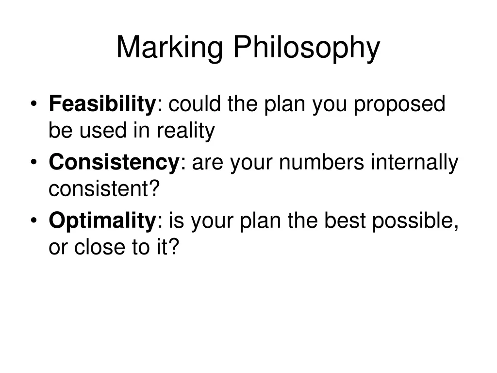
Marking Philosophy • Feasibility: could the plan you proposed be used in reality • Consistency: are your numbers internally consistent? • Optimality: is your plan the best possible, or close to it?
Example: Marking of HW1, Q5 • You submitted: • The plan: # to catch in years 0 – 30 • The consequence: NPV • We plug your plan into a correct model and check: • Feasibility: is fish population always non-negative? • Consistency: does your plan result in the NPV you reported? • Optimality: how does your NPV compare to the best possible NPV?
From the Grading Manager • Put only numbers in cells for numerical answers • 1234 • $1,234 • 1 234 Excel interprets this as text, not a number (because of the space) • 1234 fish ditto
Reminders • HW 2 due Wednesday at 11:59 pm
MGTSC 352 Lecture 4: Forecasting Methods that capture Level, Trend, and Seasonality: TES = Triple Exponential Smoothing Intro to SLR w SI = Simple Linear Regression with Seasonality Indices
Forecasting: Common Mistakes • Computing forecast error when either the data or the forecast is missing • MSE: dividing with “n” instead of “n-1” • MSE: SSE/n – 1 instead of SSE/(n – 1) • Simple methods: forgetting that the forecasts are the same for all future time periods
Recap: How Different Models Predict • Simple models: • Ft+k = Ft+1, k = 2, 3, … • DES: • Ft+k = Lt + (k Tt ), k = 1, 2, 3, … • Linear trend • TES and SLR w SI (cover today): • Ft+k = (Lt + k Tt) (Seasonality Index)
What’s a Seasonality Index (SI)? • Informal definition: SI = actual / level • Example: • Average monthly sales = $100M • July sales = $150M • July SI = 150/100 = 1.5 • SI = actual / level means: • Actual = level SI • Level = actual / SI
Works in three phases Initialization Learning Prediction Tracks three components Level Trend Seasonality TES tamed
Actual data Level Prediction Prediction Initialization Learning
Forecast = (predicted level) SI predicted level k periods into future k trend Actual data Level Prediction Time to try it out – Excel
Pg. 29 TES - Calibration (p = # of seasons) Always: UPDATED =(S) NEW + (1-S) OLD One-step Forecast: Ft+1 = (Lt + Tt) St+1-p
Level: learning phase • L(t) = LS * D(t) / S(t-p) + ( 1 - LS )*( L(t-1) + T(t-1) ) • NEW:D(t) / S(t-p) = de-seasonalize data for period t using seasonality of corresponding previous season level = actual / SI • OLD:L(t-1) + T(t-1) = best previous estimate of level for period t
Trend: learning phase • T(t) = TS * ( L(t) - L(t-1) ) + ( 1 - TS ) * T(t-1) • NEW: L(t) - L(t-1) = growth from period t-1 to period t • OLD: T(t-1) = best previous estimate for trend for period t
Seasonality: learning phase • S(t) = SS * D(t) / L(t) + ( 1 - SS ) * S(t-p) • NEW: D(t) / L(t) = actual / level SI = actual / level • OLD: S(t-p) = previous SI estimate for corresponding season 25
One-step forecasting: the past F(t+1) = [L(t) + T(t)] * S(t+1-p) "To forecast one step into the future, take the previous period’s level, add the previous period’s trend, and multiply the sum with the seasonality index from one cycle ago."
Pg. 30 k-step forecasting: the future(“real” forecast) • F(t+1) = [L(t) + k*T(t)] * S(t+1-p) • Active learning: translate the formula into English • One minute, in pairs
multiplicative seasonality additive trend TES vs SLRwSI • TES Ft+k = (Lt + k Tt) St+k-p • SLRwSI Ft+k = (intercept+ (t + k) slope) SI
TES vs SLRwSI • Both estimate Level, Trend, Seasonality • Data points are weighted differently • TES: weights decline as data age • SLRwSI: same weight for all points • Hence, TES adapts, SLRwSI does not
Patterns in the Data? • Trend: • Yes, but it is not constant • Zero, then positive, then zero again • Seasonality? • Yes, cycle of length four
TES: SE = 24.7 TES trend is adaptive SLRwSI: SE = 32.6 SLR uses constant trend Comparison
One-minute paper • Don’t put on your coat put your books away or whatnot, pull out a piece of paper instead. • Review today’s lecture in your mind • What were the two main things you learned? • What did you find most confusing? • Who is going to win the Superbowl? • Don’t put your name on the paper. • Stay in your seats for 1 minute. • Hand in on your way out