Convolution, Edge Detection, and Sampling in Image Processing
Learn about Fourier spectrum, Gaussian filtering, image scaling, aliasing, and sampling techniques in computational photography. Explore convolution, edge detection filters, image sub-sampling, and effective sampling practices for high-quality images.

Convolution, Edge Detection, and Sampling in Image Processing
E N D
Presentation Transcript
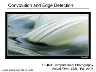
Convolution, Edge Detection, Sampling 15-463: Computational Photography Alexei Efros, CMU, Fall 2006 Some slides from Steve Seitz
Gaussian filtering • A Gaussian kernel gives less weight to pixels further from the center of the window • This kernel is an approximation of a Gaussian function:
Convolution • Remember cross-correlation: • A convolution operation is a cross-correlation where the filter is flipped both horizontally and vertically before being applied to the image: • It is written: • Suppose H is a Gaussian or mean kernel. How does convolution differ from cross-correlation?
The greatest thing since sliced (banana) bread! The Fourier transform of the convolution of two functions is the product of their Fourier transforms The inverse Fourier transform of the product of two Fourier transforms is the convolution of the two inverse Fourier transforms Convolution in spatial domain is equivalent to multiplication in frequency domain! The Convolution Theorem
2D convolution theorem example |F(sx,sy)| f(x,y) * h(x,y) |H(sx,sy)| g(x,y) |G(sx,sy)|
Low-pass, Band-pass, High-pass filters low-pass: band-pass: what’s high-pass?
The gradient direction is given by: • how does this relate to the direction of the edge? • The edge strength is given by the gradient magnitude Image gradient • The gradient of an image: • The gradient points in the direction of most rapid change in intensity
Effects of noise • Consider a single row or column of the image • Plotting intensity as a function of position gives a signal How to compute a derivative? • Where is the edge?
Look for peaks in Solution: smooth first • Where is the edge?
Derivative theorem of convolution • This saves us one operation:
Laplacian of Gaussian • Consider Laplacian of Gaussian operator • Where is the edge? • Zero-crossings of bottom graph
Laplacian of Gaussian • is the Laplacian operator: 2D edge detection filters Gaussian derivative of Gaussian
MATLAB demo g = fspecial('gaussian',15,2); imagesc(g) surfl(g) gclown = conv2(clown,g,'same'); imagesc(conv2(clown,[-1 1],'same')); imagesc(conv2(gclown,[-1 1],'same')); dx = conv2(g,[-1 1],'same'); imagesc(conv2(clown,dx,'same')); lg = fspecial('log',15,2); lclown = conv2(clown,lg,'same'); imagesc(lclown) imagesc(clown + .2*lclown)
Image Scaling This image is too big to fit on the screen. How can we reduce it? How to generate a half- sized version?
Image sub-sampling 1/8 1/4 • Throw away every other row and column to create a 1/2 size image • - called image sub-sampling
Image sub-sampling 1/2 1/4 (2x zoom) 1/8 (4x zoom) Why does this look so crufty?
Input signal: Matlab output: WHY? x = 0:.05:5; imagesc(sin((2.^x).*x)) Aj-aj-aj: Alias! Not enough samples Alias: n., an assumed name Picket fence receding Into the distance will produce aliasing…
Aliasing • occurs when your sampling rate is not high enough to capture the amount of detail in your image • Can give you the wrong signal/image—an alias • Where can it happen in images? • During image synthesis: • sampling continous singal into discrete signal • e.g. ray tracing, line drawing, function plotting, etc. • During image processing: • resampling discrete signal at a different rate • e.g. Image warping, zooming in, zooming out, etc. • To do sampling right, need to understand the structure of your signal/image • Enter Monsieur Fourier…
1/w Spatial domain Frequency domain Sampling samplingpattern w sampledsignal
w 1/w sincfunction reconstructedsignal Spatial domain Frequency domain Reconstruction
What happens when • the sampling rate • is too low?
Nyquist Rate • What’s the minimum Sampling Rate 1/w to get rid of overlaps? w 1/w sincfunction Spatial domain Frequency domain • Sampling Rate ≥ 2 * max frequency in the image • this is known as the Nyquist Rate
Antialiasing • What can be done? Sampling rate ≥ 2 * max frequency in the image • Raise sampling rate by oversampling • Sample at k times the resolution • continuous signal: easy • discrete signal: need to interpolate • 2. Lower the max frequency by prefiltering • Smooth the signal enough • Works on discrete signals • 3. Improve sampling quality with better sampling • Nyquist is best case! • Stratified sampling (jittering) • Importance sampling (salaries in Seattle) • Relies on domain knowledge
Sampling • Good sampling: • Sample often or, • Sample wisely • Bad sampling: • see aliasing in action!
Gaussian pre-filtering G 1/8 G 1/4 Gaussian 1/2 • Solution: filter the image, then subsample
Subsampling with Gaussian pre-filtering Gaussian 1/2 G 1/4 G 1/8 • Solution: filter the image, then subsample
Compare with... 1/2 1/4 (2x zoom) 1/8 (4x zoom)