Download

1 / 91
920 likes | 1.03k Views
Dive into collision detection techniques in game development. Learn the 3 phases of detection, how to handle object trajectories, configuration spaces, the Separating Axis Theorem, and the GJK Algorithm. Understand support mappings, convex hulls, and Minkowski sums in this crash course.

E N D
Physics for Games Programmers: Collision Detection Crash Course Gino van den Bergen gino@dtecta.com
Collision Detection • Track which pairs of objects… • are interpenetrating now, or ratherwill collide over the next frame if no counter action is taken. • Compute data for response.
The Problem • Object placements are computed for discrete moments in time. • Object trajectories are assumed to be continuous.
The Problem (cont’d) • If collisions are checked only for the sampled moments, some collisions are missed (tunneling). • Humans easily spot such artifacts.
The Fix • Perform collision detection in continuous 4D space-time: • Construct a plausible trajectory for each moving object. • Check for collisions along these trajectories.
Plausible Trajectory? • Use of physically correct trajectories in real-time 4D collision detection is something for the not-so-near future. • In game development real-time constraints are met by cheating. • We cheat by using simplified trajectories.
Plausible Trajectory? (cont’d) • Limited to trajectories with piecewise constant linear velocities. • Angular velocities are ignored. Rotations are considered instantaneous.
Physical Representation • Scenes may be composed of many independently moving objects. • Objects may be composed of many primitives. • Different types of primitives may be used (triangles, spheres, boxes, cylinders, capsules, andwhatnot).
Three Phases • Broad phase: Determine all pairs of objects that potentially collide. • Mid phase: Determine potentially colliding primitives of a pair of objects. • Narrow phase: Determine contact between primitives and compute response data.
Primitives • Only convex shapes are considered
Configuration Space • The configuration space obstacle of objects A and B is the set of all vectors from a point of B to a point of A.
Translation • Translation of A and/or B results in a translation of A – B.
Rotation • Rotation of A and/or B changes the shape of A – B.
Configuration Space (cont’d) • A and B intersect: A – B contains origin. • Distance between A and B: length of shortest vector in A – B.
Separating Axis Theorem • Any pair of non-intersecting polytopes has a separating axis that is orthogonal to: • a face of either polytope, or • an edge from each polytope.
Separating Axis Theorem Proof (or at least a sketch) • The CSO of non-intersecting polytopes is a polytope that does not contain the origin. • The origin lies on the outside of at least one face of the CSO. • A face of the CSO is either the CSO of a face and a vertex or the CSO of two edges.
Separating Axis Method • Test all face normals and all cross products of edge directions. • If none of these vectors yield a separating axis then the polytopes must intersect. • Given polytopes with resp. f1 and f2 faces and e1 and e2 edge directions, we need to test at most f1 + f2 +e1e2 axes.
GJK Algorithm • An iterative method for computing the distance between convex objects. • First publication in 1988 by Gilbert, Johnson, and Keerthi. • Solves queries in configuration space. • Uses an implicit object representation.
GJK Algorithm: Workings • Approximate the point of the CSO closest to the origin • Generate a sequence of simplices inside the CSO, each simplex lying closer to the origin than its predecessor. • A simplex is a point, a line segment, a triangle, or a tetrahedron.
GJK Algorithm: Workings (cont’d) • Simplex vertices are computed using support mappings. (Definition follows.) • Terminate as soon as the current simplex is close enough. • In case of an intersection, the simplex contains the origin.
Any point on this face may be returned as support point Support Mappings • A support mapping sA of an object A maps vectors to points of A, such that
Affine Transformation • Shapes can be translated, rotated, and scaled. For T(x)=Bx+c, we have
Convex Hull • Convex hulls of arbitrary convex shapes are readily available.
Minkowski Sum • Shapes can be fattened by Minkowski addition.
Basic Steps (1/6) • Suppose we have a simplex inside the CSO…
Basic Steps (2/6) • …and the point v of the simplex closest to the origin.
Basic Steps (3/6) • Compute support point w = sA-B(-v).
Basic Steps (4/6) • Add support point w to the current simplex.
Basic Steps (5/6) • Compute the closest point v’ of the new simplex.
Basic Steps (6/6) • Discard all vertices that do not contribute to v’.
Separating Axis • If only an intersection test is needed then let GJK terminate as soon as the lower bound v∙w becomes positive. • For a positive lower bound v∙w, the vector v is a separating axis.
Separating Axis (cont'd) • The supporting plane through w separates the origin from the CSO. + 0
Separating Axes and Coherence • Separating axes can be cached and reused as initial v in future tests on the same object pair. • When the degree of frame coherence is high, the cached v is likely to be a separating axis in the new frame as well. • An incremental version of GJK takes roughly one iteration per frame for smoothly moving objects.
Shape Casting • Find the earliest time two translated objects come in contact. • Boils down to performing a ray cast in the objects’ configuration space. • For objects A and B being translated over respectively vectors s and t, we perform a ray cast along the vector r = t–s onto A – B. • The earliest time of contact is
Normals • A normal at the hit point of the ray is normal to the contact plane.
GJK Ray Cast • Do a standard GJK iteration, and use the support planes as clipping planes. • Each time the ray is clipped, the origin is “shifted” to λr,… • …and the current simplex is set to the last-found support point. • The vector -v that corresponds to the latest clipping plane is the normal at the hit point.
The origin advances to the new lower bound. The vector -v is the latest normal. GJK Ray Cast (cont'd)
Accuracy vs. Performance • Accuracy can be traded for performance by tweaking the error tolerance εtol. • A greater tolerance results in fewer iterations but less accurate hit points and normals.
Accuracy vs. Performance • εtol = 10-7, avg. time: 3.65 μs @ 2.6 GHz