Download
1 / 14
140 likes | 221 Views
Explore CME initiation and propagation using data-constrained MHD simulations, comparing results to idealized models. Analyze the impact of initial conditions on CME properties and potential geoeffective effects. Future work includes validation against observations.

E N D
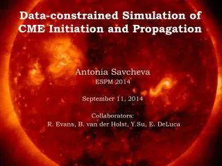
Data-constrained Simulation of CME Initiation and Propagation Antonia Savcheva ESPM 2014 September 11, 2014 Collaborators: R. Evans, B. van der Holst, Y.Su, E. DeLuca
Outline • Motivation • The flux rope insertion method • The 8 April 2010 CME • SWMF and AWSoM • Simulation set-up • Results from the simulations • Conclusions
Motivation • CME studies: • Static non-linear force-free field (NLFFF) modeling ( e.g. Savcheva & van Ballegooijen2009, Savcheva et al. 2014) • Idealized simulation with prescribed initial and/or boundary conditions (e.g. Aulanier et al. ‘10, Lugazet al.’13) • Data-constrained MHD simulations (first by Kliem et al. 2013, partial box) • Need data-constrained and data-driven simul. of CMEs
8 April 2010 region - observations • First CME observed by AIA; Hinode, STEREO data
NLFFF modelingThe flux rope insertion method • van Ballegooijen (2004) – the Coronal Modeling System (CMS) • Potential field extrapolation (data) • Insert flux rope along a filament (model) • Relax to force-free state using magnetofriction (model) • Make a grid of models, then match to observed coronal loops (data)
Models 8 April 2010 region • Modeled by Su et al. (2011) and Kliem at al. (2013) -studied stability boundary • Models with different axial flux – 4x10²⁰ - 11x1020 Mx • Unstable model with axial flux > 5x10²⁰ Mx Su et al. (2011)
The Space Weather Modeling Framework (SWMF) and AWSoM • SWMF uses BATS-R-US global MHD code • Boundary conditions – prescribed or synoptic magnetogram • Initial condition – prescribed TD of GL flux ropes, or NLFFFs • AMR, thermodynamics, resistive or ideal MHD, etc. • AWSoM – Alfven Wave Solar Model (van der Holst et al. 2014) • Starts at top of chromosphere • Stratified atmosphere • Heating by dissipation of of Alfven waves by • Reflection • Turbulent cascade
Setting-up the initial condition • Incorporate 3D grid of partial sun NLFFF model – potential field = difference field with open boundaries • Potential Source Surface Model + add potential field to difference field • Run stead state solar wind model • Set up AMR and initiate eruption in the SS SW
Comparison of CME with different initial conditions • Models with: 1) Different axial flux; 2) axial flux = 9x10²⁰ Mx with different scaling of the NLFFF-potential field 4x10²⁰ 5x10²⁰ 6x10²⁰ 7x10²⁰ 9x10²⁰ 9x1020x1.25 9x1020x2
The scaled model (NLFFF x 2) Density ratio Radial Velocity
Comparison with a TD model NLFFF TD • Same orientation and size of the initial J contour, free energy • Similar but: • Morphology differences • Speed differences • Average front velocity: • NLFFF I.C. = 1230 km/s • TD I.C. = 2000 km/s
Height-time and velocity-time plots • Measure where density is 4% above background -> get front of CME, measure velocity of front 9x1020 x 2 9x1020 x 1.25 TD corr. 9x1020 x2
Conclusions and future work • The first data-constrained global CME simulation from realistic initial and boundary conditions • Explored the effect of the initial condition’s axial flux on the CME properties • Compared to a TD idealized simulation and showed differences • Computed height-time and velocity-time plots • Future: • Compare the H-t, V-t plots and simulated white light images to observations • Propagate a geoeffective CME to 1AU and simulate signatures at Earth and STEREO – 7 Aug 2010