Download
1 / 27
270 likes | 462 Views
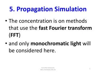
5. Propagation Simulation. The concentration is on methods that use the fast Fourier transform ( FFT ) and only monochromatic light will be considered here. 5.1 Fresnel Transfer Function (TF) Propagator.

E N D
5.Propagation Simulation • The concentration is onmethods that use the fast Fourier transform (FFT) • and only monochromatic lightwill be considered here. Kun Shan University htto://www.ksu.edu.tw
5.1 Fresnel Transfer Function (TF) Propagator • The Fresnel diffraction expression is often the approach of choice forsimulations since it applies to a wide range of propagation scenarios and isrelatively straightforward to compute. Kun Shan University htto://www.ksu.edu.tw
the transfer function H given by • Start a New M-file and save it with name “propTF” Enter the followingfunction: Kun Shan University htto://www.ksu.edu.tw
This propagator function takes the source field u1 and produces the observation field u2 where the source and observation side lengths and sample coordinates are identical. • Here are a few remarks on propTF with associated line numbers: • (a) Line 11: The size function finds the sample dimensions for the input field matrix u1 (only M is used). This helps reduce the number Kun Shan University htto://www.ksu.edu.tw
(b) Line 16: A line is saved by using fx twice in the meshgrid command since fy would be the same. • (c)Line 18: The transfer function H of Eq. (5.2) is programmed, although the exp(jkz) term is ignored. This term doesn’t affect the transverse spatial structure of the observation plane result. • (d)Line 19: H is created in the array center but is shifted (fftshift) before the FFT. Kun Shan University htto://www.ksu.edu.tw
(e) Line 20: Similarly, the source field u1 is assumed to be in the array center; so, fftshift is applied before the 2D FFT is computed. • (f) Line 21: U1 is multiplied “pointwise” by the transfer function H and the inverse FFT is computed to complete the convolution. • (g) Line 22: Finally, ifftshift centers u2 for display. Kun Shan University htto://www.ksu.edu.tw
5.2 Fresnel Impulse Response (IR) Propagator • A propagation approach impulse response h Kun Shan University htto://www.ksu.edu.tw
1 function[u2]=propIR(u1,L,lambda,z); 2 % propagation - impulse response approach 3 % assumes same x and y side lengths and 4 % uniform sampling 5 % u1 - source plane field 6 % L - source and observation plane side length 7 % lambda - wavelength 8 % z - propagation distance 9 % u2 - observation plane field 10 11 [M,N]=size(u1); %get input field array size 12 dx=L/M; %sample interval 13 k=2*pi/lambda; %wavenumber 14 15 x=-L/2:dx:L/2-dx; %spatial coords 16 [X,Y]=meshgrid(x,x); 17 18 h=1/(j*lambda*z)*exp(j*k/(2*z)*(X.^2+Y.^2)); %impulse 19 H=fft2(fftshift(h))*dx^2; %create trans func 20 U1=fft2(fftshift(u1)); %shift, fft src field 21 U2=H.*U1; %multiply 22 u2=ifftshift(ifft2(U2)); %inv fft, center obs field 23 end Kun Shan University htto://www.ksu.edu.tw
(a) Line 18: h is implemented, and the FFT is applied to get H. • (b) Line 19: Note the multiplier dx^2 for H. The FFT of u1 and FFT−1 of U2take care of each other’s scaling, but the FFT of h needs its own scaling. Kun Shan University htto://www.ksu.edu.tw
5.3 Square Beam Example • Now it is time to try out the TF and IR propagators. Consider a source plane withdimensions 0.5 m × 0.5 m (L1 = 0.5 m). Start a New M-file and use the name“sqr_beam.” Enter the following: Kun Shan University htto://www.ksu.edu.tw
1 % sqr_beam propagation example 2 % 3 L1=0.5; %side length 4 M=250; %number of samples 5 dx1=L1/M; %src sample interval 6 x1=-L1/2:dx1:L1/2-dx1; %src coords 7 y1=x1; Variables with “1” are source plane quantities. The source and observation planeside lengths are the same for the TF and IR propagators, i.e., L1 = L2 = L, but thisis not true for other propagators, so the variable L1 is retained here. The codesets up 250 samples across the linear dimension of the source plane, and thesample interval dx1 works out to be 2*10^−3 m (2 mm). Kun Shan University htto://www.ksu.edu.tw
Assume a square aperture with a half width of 0.051 m (51 mm) illuminated • by a unit-amplitude plane wave from the backside, where λ= 0.5 μm. • Thesimulation, therefore, places 51 samples across the aperture, which provides agood representation of the square opening (see Section 2.2). Add the followingcode: Kun Shan University htto://www.ksu.edu.tw
8 lambda=0.5*10^-6; %wavelength 9 k=2*pi/lambda; %wavenumber 10 w=0.051; %source half width (m) 11 z=2000; %propagation dist (m) 12 13 [X1,Y1]=meshgrid(x1,y1); 14 u1=rect(X1/(2*w)).*rect(Y1/(2*w)); %src field 15 I1=abs(u1.^2); %src irradiance 16 % 17 figure(1) 18 imagesc(x1,y1,I1); 19 axis square; axis xy; 20 colormap('gray'); xlabel('x (m)'); ylabel('y (m)'); 21 title('z= 0 m'); Kun Shan University htto://www.ksu.edu.tw
Source plane irradiance for sqr_beam propagation simulation Kun Shan University htto://www.ksu.edu.tw
The propagation distance z is 2000 m, so the Fresnel number for this case is NF =w2/λz = 2.6, which is reasonable for applying the Fresnel expression. • The sourcefield is defined in the array u1. The irradiance is found by squaring the absolutevalue of the field. Executing this script generates Fig. 5.1, which verifies thesource plane arrangement. Kun Shan University htto://www.ksu.edu.tw
22 u2=propTF(u1,L1,lambda,z); %propagation 23 24 x2=x1; %obs coords 25 y2=y1; 26 I2=abs(u2.^2); %obs irrad 27 28 figure(2) %display obs irrad 29 imagesc(x2,y2,I2); 30 axis square; axis xy; 31 colormap('gray'); xlabel('x (m)'); ylabel('y (m)'); 32 title(['z= ',num2str(z),' m']); 33 % 34 figure(3) %irradiance profile 35 plot(x2,I2(M/2+1,:)); 36 xlabel('x (m)'); ylabel('Irradiance'); 37 title(['z= ',num2str(z),' m']); 38 % Kun Shan University htto://www.ksu.edu.tw
39 figure(4) %plot obs field mag 40 plot(x2,abs(u2(M/2+1,:))); 41 xlabel('x (m)'); ylabel('Magnitude'); 42 title(['z= ',num2str(z),' m']); 43 % 44 figure(5) %plot obs field phase 45 plot(x2,unwrap(angle(u2(M/2+1,:)))); 46 xlabel('x (m)'); ylabel('Phase (rad)'); 47 title(['z= ',num2str(z),' m']); Kun Shan University htto://www.ksu.edu.tw
Now try the impulse response IR propagator. Change line 22 to u2=propIR(u1,L1,lambda,z); %propagation and run sqr_beam. The results in this case should be identical to those in Figs.5.2 and 5.3. Kun Shan University htto://www.ksu.edu.tw
Figure 5.2 Observation plane irradiance (a) pattern and (b) profile. Kun Shan University htto://www.ksu.edu.tw
Figure 5.3 Observation plane (a) magnitude and (b) phase profiles. Kun Shan University htto://www.ksu.edu.tw
5.4 Fresnel Propagation Sampling • 5.4.1 Square beam example results and artifacts In Fig. 5.4 both propTF and propIR results are shown for the sqr_beam routine at propagation distances ranging from 1000 to 20,000 m. Kun Shan University htto://www.ksu.edu.tw