Download
1 / 8
120 likes | 406 Views
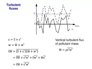
Turbulent fluxes. Vertical turbulent flux of pollutant mass. Turbulent stress. Vertical fluxes of momentum, heat, water vapor, and pollutant. Gradient-transport (K-theory).

E N D
Turbulent fluxes Vertical turbulent flux of pollutant mass
Turbulent stress Vertical fluxes of momentum, heat, water vapor, and pollutant
Gradient-transport (K-theory) Km, Kh, and Kz are called the eddy diffusivities or exchange coefficients of momentum, heat, and mss, respectively. (Km is also called eddy or turbulent viscosity). The gradient-transport (K-theory) relations are not based on any rigorous theory, but only on an intuitive analogy between molecular and turbulent exchange processes.
Prandtl’s mixing length theory From dimensional analysis, we recognizing that eddy diffusivity must be a product of appropriate length and velocity scales. In the surface layer (constant flux layer) k= 0.40 is thevon Karman constant is the friction velocity that is related to surface stress Finally, we have
In the surface layer, under neutral condition, we have: We can define a surface roughness parameter such that at , . Therefore, we can obtain the well-known logarithmic velocity profile law, that is
FIRST-ORDER PARAMETERIZATION OF TURBULENT FLUX Time-averaged envelope Near-Gaussian profile • Observed mean turbulent dispersion of pollutants is near-Gaussian eparameterize it by analogy with molecular diffusion: z Instantaneous plume Source <C> Turbulent diffusion coefficient • Typical values of Kz: 102 cm2s-1 (very stable) to 107 cm2 s-1 (very unstable); mean value for troposphere is ~ 105 cm2 s-1 • Same parameterization (with different Kx, Ky) is also applicable in horizontal direction but is less important (mean winds are stronger)
Mass conservation and diffusion equation If U=0, the diffusion equation can be simplified to For an instantaneous point source, the solution of the above equation is Q is the total mass of pollutant in the puff
TYPICAL TIME SCALES FOR VERTICAL MIXING • Estimate time Dt to travel Dz by turbulent diffusion: tropopause (10 km) 10 years 5 km 1 month 1 week 2 km “planetary boundary layer” 1 day 0 km