Multiple Regression Analysis: Redefining Variables and Functional Form

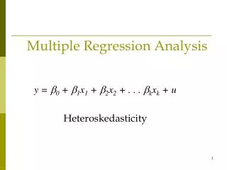
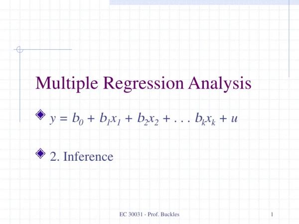
1. Multiple Regression Analysis y = b0 + b1x1 + b2x2 + . . . bkxk + u 4. Further Issues

2. Redefining Variables • Suppose we have a model with a variable like income measured in dollars on the left-hand-side. Now we re-define income to be measured in tens of thousands of dollars. What effect will this have on estimation and inference? • It will not affect the R2 • Will such scaling have any effect on t-stats, F-stats and confidence intervals? • No, these will also have the same interpretation • Changing the scale of the y variable just leads to a corresponding change in the scale of the coefficients

3. Redefining Variables (cont) • Suppose we originally obtain • In this specification, house price is measured in dollars. • What happens if we re-estimate this with house price measured in thousands of dollars?

4. Redefining Variables (cont) • If we measure price in thousands of dollars, the new coefficient will be the old coefficient divided by 1000 (same estimated effect!) • The standard errors will be 1000 times smaller • t-stats etc. will be identical

5. Redefining Variables (cont) • Changing the scale of one of the x variables:What if we redefine square feet as thousands of square feet? Now all the ’s have the same interpretation as before with the exception of 1-hat • It will be 1000 times larger • Why? Because now a 1 unit change in square feet is the same as what previously was a 1000 unit change in square feet. • The standard error will also be 1000 times larger and t-stats etc. will have the same interpretation

6. Functional Form • OLS can be used for relationships that are not strictly linear in x and y by using nonlinear functions of x and y – will still be linear in the parameters Example: log(wage)= 0 +1(educ)+2(exper)+3 (exper)2 In this particular specification we have an example of a log specification with a quadratic term--both are examples of nonlinearities that can be introduced into the standard linear regression model

7. Interpretation of Log Models 1. If the model is ln(y) = b0 + b1ln(x) + u, then b1 is an elasticity. e.g. if we obtained an estimate of 1.2, this would suggest that a 1 percent increase in x causes y to increase by 1.2 percent. 2. If the model is ln(y) = b0 + b1x + u, then b1*100 is the percent change in y resulting from a unit change in x. e.g. if we obtained an estimate of 0.05, this would suggest that a 1 unit increase in x causes a 5% increase in y. 3. If the model is y = b0 + b1ln(x) + u, then b1/100 is the unit change in y resulting from a 1 percent change in x. e.g. if we obtained an estimate of 20, this would suggest that a 1 percent increase in x causes a 0.2 unit increase in y.

8. Why use log models? • Log models are invariant to the scale of the variables since we’re measuring percent changes • They can give a direct estimate of elasticity • For models with y > 0, the conditional distribution is often heteroskedastic or skewed, while ln(y) is much less so • The distribution of ln(y) is more narrow, limiting the effect of outliers

9. Some Rules of Thumb What types of variables are often used in log form? *Variables in positive dollar amounts *Variables measuring numbers of people -school enrollments, population, # employees *Variables subject to extreme outliers What types of variables are often used in level form? *Anything that takes on a negative or zero value *Variables measured in years

10. Quadratic Models • Captures increasing or decreasing marginal effects • For a model of the form y = b0 + b1x + b2x2 + u, we can’t interpret b1 alone as measuring the change in y with respect to x. Now the effect of an extra unit of x on y depends in part on the value of x. Suppose b1 is positive. Then if b2 is positive, an extra unit of x has a larger impact on y when x is big than when x is small. If b2 is negative, an extra unit of x has a smaller impact on y when x is big than when x is small.

11. More on Quadratic Models • Suppose that the coefficient on x is positive and the coefficient on x2 is negative • Then y is increasing in x at first, but will eventually turn around and be decreasing in x • We may want to know the point of inflection

12. More on Quadratic Models • Suppose that the coefficient on x is negative and the coefficient on x2 is positive • Then y is decreasing in x at first, but will eventually turn around and be increasing in x

13. Interaction Terms • We might think that the marginal effect of one RHS variable depends on another RHS variable Example: suppose the model can be written: y = b0 + b1x1 + b2x2 + b3x1x2 + u • Where y is house price, x1 is the number of square feet and x2 is the number of bedrooms. • So the effect of an extra bedroom on price is

14. Interaction Terms • If b3>0, this tells us that an extra bedroom boosts the price of a house more, if the square footage of the house is higher. • This shouldn’t be surprising. After all, an extra bedroom in a small house is likely to be small compared with an extra bedroom in a large house. So we would expect an extra bedroom in a big house to be worth more. • Note that this makes interpretation of b2 a bit less straightforward. • Technically, b2 tells us how much an extra bedroom is worth in a house with zero square feet. • It may be useful to report on the value of b2+b3x1 for the mean value of x1 .

15. More on Goodness-of-Fit: Adjusted R-Squared • Recall that the R2 will always increase as more variables are added to the model • The adjusted R2 takes into account the number of variables in a model, and may decrease • The usual R2 can be written:

16. Adjusted R-Squared (cont) • We can define the “population R-squared” as • We can use SSR/(n-k-1) as unbiased estimate ofu2 • Similarly can use SST/(n-1) as unbiased estimate of y2 • Therefore, adjusted R2 “R-bar squared” is:

17. Adjusted R-Squared (cont) • Notice that R-bar squared can go up or down when a variable is added, unlike the regular R-squared which always goes up • R-bar squared is not necessarily “better”- the ratio of 2 unbiased estimators isn’t necessarily unbiased • Better to treat it as an alternative way of summarizing goodness of fit • If you add a variable to the RHS and the R-bar squared doesn’t rise, this is likely (though not surely) an indication it shouldn’t be included in the model

18. Comparing Nested Models • Suppose you wanted to compare the following two models: 1. y=0+1x+u 2. y=0+1x+2x2+ u We say that (1) is nested in (2); alternatively, (1) is a special case of (2). With a t-test on 2 we can choose between these two models (if reject null of 2=0, we pick model 2). For multiple exclusion restrictions can use F-test.

19. Comparing Non-Nested Models • Suppose you wanted to compare the following two models: 1. y=0+1log(x)+ 2. y=0+1x+ 2x2+  • One is not nested in the other, so t-test or F-test cannot be used to compare. • Here R-bar-squared can be useful. We can simply choose the model with the higher R-bar-squared. • Note that a simple comparison of regular R-squared would tend to lead us to choose the model with more explanatory variables. • Note that if the LHS variable takes a different form between (1) and (2) we cannot compare using R-bar-squared (or R-squared).

20. Goodness of Fit • Important not to fixate too much on adj-R2 and lose sight of theory and common sense • If economic theory clearly predicts a variable belongs, generally leave it in • Don’t want to exclude a variable that prohibits a sensible interpretation of the variable of interest • Remember the ceteris paribus interpretation of multiple regression

21. Residual Analysis • Sometimes looking at the residuals (i.e. predicted - observed) provides useful information • Example: Regress price of cars on characteristics • Engine size, efficiency, luxury amenities, roominess, fuel efficiency, etc. • Then the residual = actual price - predicted price • By picking the car with the lowest (most negative) residual, you would be choosing the most underpriced car (assuming you’re controlling for all relevant characteristics)

22. Standard Errors for Predictions • Suppose we want to use our estimates to obtain a specific prediction. • Such predictions are subject to sampling variation because they are functions of estimated parameters • First, suppose that we estimate: y=0+1x1+2x2+3x3+4x4+…+u and we want to obtain a prediction of y for specific value of the x’s. In general we can obtain predictions of y by plugging values of the actual x’s into our fitted model.

23. Standard Errors for Predictions • Let c1, c2, …, ck denote particular values of the x variables, for which we want to obtain a prediction of y. • We can think of estimating a parameter • A good estimator is

24. Predictions (cont) • To get a confidence interval for our estimate of q0 we need its standard error • Like testing a linear combination of parameters, the difficulty is getting this standard error • Can rewrite as b0 = q0 – b1c1 – … – bkck and plug this into y=0+1x1+…+kxk+u to get • If we regress y on a constant and on (x1– c1),…, (xk– ck) we will obtain an estimate of q0 and the standard error of that estimate. This can be used to construct a confidence interval.

25. Predictions (cont) • The standard error we obtain here is for the expected value of y given particular x values.. This can be thought of as the standard error of the average y value for the sub-population that has those exact x characteristics. It is not the same as a standard error for a prediction about a particular individual from the population. • In order to form a confidence interval for a particular individual we need to also take into account the variance in the unobserved error. • Let y0 = some outcome for which we want a confidence interval (for some individual in the population who you wish to make predictions about), x0 = new values of independent variables, and u0 be the unobserved error. Then,

26. Predictions (cont) • The best prediction of y0 is: • The prediction error is: • We know that (because our estimators are unbiased)

27. Predictions (cont) • There are 2 sources of variation: 1. Variance due to the sampling error in prediction (because yhat based on estimated coefficients) 2. Variance in the error of the population

28. Prediction interval • We can estimate the standard error of prediction:

29. Predicting y in a log model • For the prediction • Simple exponentiation of the predicted ln(y) will underestimate the expected value of y • Use caution when making predictions in a model with ln(y) on LHS (see text pages 219-221).