Chapter 1: What is the Mesoscale?
110 likes | 299 Views
Chapter 1: What is the Mesoscale?. Mesoscale energy sources. (1) Scales of atmospheric motion. k = 1/ l. Note two spectral extremes: (a) A maximum at about 2000 km (b) A minimum at about 500 km. [shifted x10 to right]. inertial subrange ( Kolmogorov 1941). power spectrum

Chapter 1: What is the Mesoscale?
E N D
Presentation Transcript
Chapter 1: What is the Mesoscale? Mesoscale energy sources
(1) Scales of atmospheric motion k = 1/l Note two spectral extremes: (a) A maximum at about 2000 km (b) A minimum at about 500 km [shifted x10 to right] inertial subrange (Kolmogorov 1941) power spectrum units: m2 s-2 per wavenumber (m-1) bin 1 100 10 1000 wavelength [km] Gage and Nastrom (1985)
energy cascade Big whirls have little whirlsthat feed on their velocity;and little whirls have lesser whirls,and so on to viscosity. -Lewis Fry Richardson FA=free atmos. BL=bound. layer L = long waves WC = wave cyclones TC=tropical cyclones cb=cumulonimbus cu=cumulus CAT=clear air turbulence From Ludlam (prior to Gage/Nastrom) mesoscale
Scales of atmospheric motion • Air motions at all scales from planetary-scale to microscale explain weather: • planetary scale: low-frequency (10 days – intraseasonal) e.g. MJO, blocking highs (~10,000 km) – explains low-frequency anomalies • size such that planetary vortadv > relative vortadv • hydrostatic balance applies • synoptic scale: cyclonic storms and planetary-wave features: baroclinic instability (~3000 km) – deep stratiform clouds • size controlled by b=df/dy • hydrostatic balance applies • mesoscale: waves, fronts, thermal circulations, terrain interactions, mesoscale instabilities, upright convection & its mesoscale organization: various instabilities – synergies (10-500 km) – stratiform & convective clouds • time scale between 2p/N and 2p/f • hydrostatic balance usually applies • microscale: buoyant eddies (cumuli, thermals), turbulence: static and shear instability(1-5 km) – convective clouds • Size controlled by entrainment and perturbation pressures • no hydrostatic balance buoyancy: 2p/N ~ 2p/10-2 ~ 10 minutes inertial: 2p/f = 12 hours/sin(latitude) = 12 hrs at 90°, 24 hrs at 30°
Eulerian vs Lagrangian • Eulerian time scale te: time for system to pass, assuming no evolution • te=L/U , where L is size, U is basic wind speed • Lagrangian time scale tl : time for particle to travel through system • for tropical cyclone or tornado, • for sea breezes, • for internal gravity waves, • LagrangianRossby number: intrinsic frequency / Coriolis parameter • Rol= 1 for inertial oscillations, but Rol>>1 for buoyancy oscillations • Rossby radius of deformation: • see COMET module “the balancing act of geostrophic adjustment”
L geostrophic adjustment: principle
1.2 Mesoscale vs. synoptic scale Fig. 1.2 (Fujita 1992)
1.2 Mesoscale vs. synoptic scale 24 hr radar loop Storm Predictions Center Meso-analysis page Fig. 1.3
1.2 Mesoscale vs. synoptic scale Ro≥1 for mesoscale flow The aspect ratio (D/L) determines whether hydrostatic balance applies 1.2.1 gradient wind balance 1.2.2 hydrostatic balance on chalkboard key results: Fig. 1.4