Download
1 / 36
360 likes | 468 Views
Investigating wintertime Arctic surface field biases in CCM, CAM, and CCSM simulations, exploring hypotheses and solutions using a linear model approach. Analyzing the impact of topography, surface drag, and resolution on model biases.

E N D
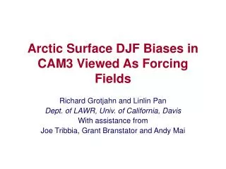
Forcing Fields Derived from Arctic Surface Biases in CAM3 Richard Grotjahn and Linlin Pan Dept. of LAWR, Univ. of California, Davis With assistance from Grant Branstator and Joe Tribbia
Introduction • Biases in wintertime Arctic surface fields have resisted model improvements and are similar in CCM, CAM, and CCSM runs. • Sea level pressure (SLP) is: • too low in the Beaufort Sea • too high (or less low depending on the model and version) in the Barents Sea. • too low in N. Atlantic, Baltic, W. Russia • SLP bias is also strongly linked to topography, especially Greenland
Is the bias an NAO or AO? • Superficial similarity, but probably not. • The model’s fundamental SLP EOF has only a small projection onto the SLP bias. Bias with leading eof removed Leading EOF bias
Some Hypotheses • Frequency and Intensity of mid-latitude frontal cyclones:The stationary wave model solutions forced by transient eddy fluxes and associated diabatic heating extends into the Arctic region. Compared to observations, recent versions of NCAR models tend to have too many and too intense frontal cyclones. • Surface drag:Surface roughness and boundary layer drag over Alaska and Eastern Siberia may be too small (no difference between flat plain and mountainous regions) allowing too much low-level flow between Arctic and northern Pacific. • Topography:Similar to surface drag in that interaction with the Pacific may be too easy. In this case, ‘small’ mountain ranges in Eastern Siberia and Alaska (such as the Brooks range) are poorly resolved including their envelope height. • Resolution on the spherical surface:Model (grid) may be tuned for middle latitudes and tropics, higher resolution in Arctic may cause misrepresentation of SLP (and other variables) over Arctic region.
Linear Model to Study Bias • Linear model (Branstator, 1990) to calculate forcing sufficient to generate parts of the bias field. • Model variables: T, ζ, Div, Q (ln of sfc pres.) • Model used two ways: • Input bias field and find forcing. Can input subset of bias • Input forcing and find solution. Can use subsets of the forcing. • Similar general features are found in the bias if NCEP/NCAR Renalysis 1 or ERA-40 data are used. • Bias used is balanced • R12 with 10 levels to be shown Q=ln(Ps)
Bias in linear model Vorticity • Linear model balanced bias construction • Temperature bias is the model NCEP/NCAR reanalysis 1 difference. • Vorticity bias is derived from geostrophic winds calculated from the bias in geopotential. • Divergence bias is calculated from geostrophic winds and Ekman pumping associated with the vorticity bias (the latter mainly influences the boundary layer). • Log of surface pressure (Q=ln(Ps)) bias is derived from SLP after filtering to the topographic resolution of the linear model. SLP and Ps have similar dominant features except the results from using SLP are more smooth. Divergence Temperature Q=ln(Ps)
Global Forcing in Linear Model Vorticity • Forcing fields deduced from the bias have obvious dipole structures in Q, vorticity, and temperature forcing fields that straddle high topography. • Dipole associated with the Tibetan plateau removed by removing forcing south of 30oN. Divergence Temperature Q=ln(Ps)
Forcing North of 30 N Vorticity • Forcing fields deduced from the bias have obvious dipole structures in Q, vorticity, and temperature forcing fields that straddle high topography. • Dipole associated with the Tibetan plateau removed by removing forcing south of 30oN. Divergence Temperature Q=ln(Ps)
Solution for forcing North of 30 N Vorticity • Ignoring forcing south of 30N still has solutions similar to the bias in Arctic • Divergence forcing here is solely from geostrophic wind Divergence Temperature Q=ln(Ps)
Solution (Ekman) for forcing N of 30 N Vorticity • Adding Ekman pumping diminishes importance of the divergence forcing. • Divergence forcing here is from Ekman pumping with geostrophic wind alters divergence and near surface vorticity solutions, but has little effect upon T or Q (SLP). • T and Q solutions not sensitive to the diffusion coefficient. Vorticity sensitive at low levels. • K=5 m2s-1 shown. Divergence Temperature Q=ln(Ps)
Subregions of forcing field • A subregion of the total forcing field is selected in a region of interest linked to specific features in the Arctic bias • North Atlantic region of dipole bias: low SLP over North Sea to Eastern Europe, high SLP over Barents Sea • Beaufort region: low SLP over Beaufort Sea • The solution is compared with the model bias
North Atlantic Local Forcing Vorticity • Forcing fields in 90W – 50E, 50N – pole. (value reduced to zero over last 15o) Divergence Temperature Q=ln(Ps)
North Atlantic Local Forcing Solution Vorticity • Forcing fields in 90W – 50E, 50N – pole. (value reduced to zero over last 15o) • Bias-like solutions Divergence Temperature Q=ln(Ps)
Beaufort Local Forcing Vorticity • Forcing fields in 100E – 120W, 50N – pole. (value reduced to zero over last 15o) Divergence Temperature Q=ln(Ps)
Beaurfort Local Forcing Solution Vorticity • Forcing fields in 100E – 120W, 50N – pole. (value reduced to zero over last 15o) • Bias-like solutions Divergence Temperature Q=ln(Ps)
Subregions of bias • A subregion of the total bias is selected in a region of interest linked to specific features in the Arctic bias • North Atlantic region of dipole bias: low SLP over North Sea to Eastern Europe, high SLP over Barents Sea • Beaufort region: low SLP over Beaufort Sea • Forcing for that subregion of bias found • Solution for that forcing found and compared with model bias
North Atlantic Local Bias Vorticity • Forcing fields in 100W – 80E, 30N – pole. (value reduced to zero over last 15o) Divergence Q=ln(Ps) Temperature
Forcing from North Atlantic Local Bias Vorticity • Forcing based on bias in subregion from 100W – 80E, 30N – pole. (value reduced to zero over last 15o) Divergence Q=ln(Ps) Temperature
North Atlantic Local Bias Solution Vorticity • Bias fields in subregion from 100W – 80E, 30N – pole. (value reduced to zero over last 15o) • Bias-like solutions recapture the dipolar SLP structure. Divergence Q=ln(Ps) Temperature
Q=ln(Ps) North Atlantic Local Bias Forcing E-W @ 55N E-W @ 75N Vorticity N-S @ 15W • Bias subregion from 100W – 80E, 30N – pole forcing solution • Forcing fields: • Equivalent barotropic in vorticity, • Baroclinic (N-S and E-W) in temperature Divergence Temperature
Q=ln(Ps) North Atlantic Local Bias Solution E-W @ 55N E-W @ 75N Vorticity N-S @ 15W • Bias subregion from 100W – 80E, 30N – pole forcing solution • Bias-like solutions: • Equivalent barotropic in vorticity, • Baroclinic in temperature Divergence Temperature
Beaufort Local Bias Vorticity • Forcing fields in 100E – 125W, 50N – pole. (value reduced to zero over last 15o) Divergence Q=ln(Ps) Temperature
Forcing from Beaufort Local Bias Vorticity • Forcing based on bias in subregion from 100E – 125W, 50N – pole. (value reduced to zero over last 15o) Divergence Q=ln(Ps) Temperature
Beaufort Local Bias Solution Vorticity • Bias fields in subregion from 100E – 125W, 50N – pole. (value reduced to zero over last 15o) • Bias-like solutions recapture the dipolar SLP structure. Divergence Q=ln(Ps) Temperature
Q=ln(Ps) Beaufort Local Bias Forcing Vorticity • Bias subregion from 100W – 80E, 30N – pole forcing solution • Forcing fields: (pattern ‘opposite’ to N. Atlantic cross sections) • Baroclinic (N-S and E-W) in vorticity, • Barotropic in temperature Divergence E-W @ 75N N-S @ 160E Temperature
Q=ln(Ps) Beaufort Local Bias Solution Vorticity • Bias subregion from 100W – 80E, 30N – pole forcing solution • Forcing fields: (pattern ‘opposite’ to N. Atlantic cross sections) • Equivalent barotropic in vorticity, • Stratosphere in temperature – model too warm Divergence E-W @ 75N N-S @ 160E Temperature
.nc files of bias, forcing, & solution • Files are available for anyone to look at in netcdf format for easy use of ncl, IDV, ferret, etc. • Link is: http://atm.ucdavis.edu/~lpan/doc/
Summary & Tentative Conclusions • Linear model used to investigate forcing and CAM model bias • The linear model reproduces structure and magnitudes of the 3 main near-Arctic features of interest in the bias field: • Low SLP over N Europe • High SLP over Barents Sea • Low SLP over Beaufort Sea • Forcing fields suggest first two are linked. • Regional subsets were tested: • Subset of global forcing from global bias solution similar to bias • Subset of bias forcing solution similar to bias feature • Forcing for these two situations is somewhat different. • Solutions from latter much better than from former • Dipole in forcing associated with monopole in solution (or input bias) • Bias not related to NAO/AO • North Atlantic (from input subset of bias): • Forcing: baroclinic T, eq barotropic Vort. Bias: baroclinc in T, eq. barotropic Vort • Beaufort (from input subset of bias): • Forcing: eq. barotropic T, baroclinic Vort. Bias: stratosphere in T, eq. barotropic Vort • Future work: Building 64bit machine now to allow higher horizontal resolution. • The key question: what phenomena (or misrepresented phenomena) cause these forcing patterns?
End • Thanks!
Introduction • Biases in wintertime Arctic surface fields have resisted model improvements and are similar in CCM, CAM, and CCSM runs. • Sea level pressure (SLP) is too low in the Beaufort and North Seas and too high (or less low depending on the model and version) in the Barents Sea. SLP bias is also strongly linked to topography, especially Greenland.
Introduction Vorticity σ=0.95 • Linear model (Branstator, 1990) to calculate forcing sufficient to generate parts of the bias field. • Model variables: T, ζ, Div, Q (ln of sfc pres.) • Model used two ways: • Input bias field and find forcing. Can input subset of bias • Input forcing and find solution. Can use subsets of the forcing. • Bias used is balanced • Similar general features are found in the bias if NCEP/NCAR Renalysis 1 or ERA-40 data are used. • R12 with 10 levels to be shown Divergence σ=0.95 Temperature σ=0.95 Q=ln(Ps)
Q=ln(Ps) North Atlantic Local Bias Forcing E-W @ 55N E-W @ 75N Vorticity N-S @ 15W • Bias subregion from 100W – 80E, 30N – pole forcing solution • Forcing fields: • Equivalent barotropic in vorticity, • Baroclinic (N-S & E-W) in temperature Divergence Temperature
Q=ln(Ps) North Atlantic Local Bias Solution E-W @ 55N E-W @ 75N Vorticity N-S @ 15W • Bias subregion from 100W – 80E, 30N – pole forcing solution • Bias-like solutions: • Equivalent barotropic in vorticity, • Baroclinic in temperature Divergence Temperature