Download
1 / 22
220 likes | 341 Views
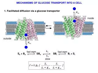
k 1. fast eqm. fast eqm. S e + B e SB e SB i B i + S i. k -1. slow. MECHANISMS OF GLUCOSE TRANSPORT INTO A CELL. 1. Facilitated diffusion via a glucose transporter. K m. inside. outside. K m.

E N D
k1 fast eqm fast eqm Se + Be SBe SBi Bi + Si k-1 slow MECHANISMS OF GLUCOSE TRANSPORT INTO A CELL 1. Facilitated diffusion via a glucose transporter Km inside outside Km
MECHANISMS OF GLUCOSE TRANSPORT INTO A CELL 2. Simple diffusion inside outside slow fast eqm fast eqm
Comparison of simple and facilitated diffusion in terms of initial rates simple facilitated Initial rates (Si = 0) Jmax = kBTwhen Se >> Km Initial rate behavior clearly distinguishes simple from facilitated diffusion mechanisms In terms of Jmax
THE EXPERIMENTAL RESULT WE ARE TRYING TO EXPLAIN “tracer” analysis with 14C glucose 1 f, fraction of equilibrium concentraiton inside chemical analysis of glucose To see if this behavior can be accounted for by either mechanism, we will express the rate equations in terms of f, the fraction of equilibrium concentration inside the cell (the y axis on the plot)
Express the flux in terms of f, the fractional approach to equilibrium (Se does not change much during approach to equilibrium) ne Define the fractional approach to equilibrium, f ni Vin Vout Vout >> Vin For simple diffusion Jmax is at f = 0 Jmax = PKbSe
Facilitated diffusion Divide numerator and denominator of flux equation by Se
facilitated diffusion Simple diffusion Relative flux at Km/Se = 0.1 (transporter sites saturated) Only halfway to equilibrium, the flux of the facilitated diffusion has dropped to 8% of its maximum value, while the simple diffusion continues at 50% of its maximum. Why is the facilitated process so slow here? f = Si/(Si)eqm
Se/Km This result can account for the anomalous rapid equilibration of “tracer” glucose while the chemical equilibration is slow. The tracer is in very low concentration, well below saturation. In this case, the efflux is not saturated, and much slower than the influx. Although the net flux is rather low due to low Se, it does not have far to go to reach equilibrium. This is most easily seen by determining the time dependence of f.
NUMERICAL SOLUTION TO THE FLUX EQUATION: time dependence of Si Vi = cell internal volume Si in molecules/cm3 Divide through by Se f = Si/Se Where r = radius of a spherical cell Can be solved numerically for f = f(t) for particular choices of Se, Km, r, BT, k
NUMERICAL SOLUTION TO THE FLUX EQUATION: time dependence of f Spherical cell of r = 5mm Km = 1x10⁻³ Molar k= 200 molecules s-1 3/r = A/V = 6 x 103 cm-1 BT = 1011 transporters cm2 (surface/volume of cell) Tracer experiment has very low effective Se! Even in the presence of a large excess of unlabeled glucose, the equilibration of tracer is fast. f = Si/Se = Si/(Si)eqm Chemical analysis experiment has high Se
Appendix 1. Derivation of the flux equation for facilitated diffusion Start with (1) Let ye and yi be the fractions of carrier sites at each surface that are complexed with S: (2) Where BTe and BTi are the total concentrations of binding sites at the external and internal surfaces, respectively, ie (3) Thus, (4) Now define the dissociation constant of S from the carrier as (5) On rearrangement (6)
Substitution of Be, Bi from (6) into (4) (7) Using (7) and (2) (8) Substituting (8) into (1) (9) If we assume that the binding sites on the transporter are randomly distributed between the two faces of the membrane (10) Finally, (9) and (10) give
Summary so far: 1. Empirical (experimental) rate law: Rate = k[A]m[B]n 2. Methods for determining the empirical rate law: initial rates; integrated rate laws. 3. Rate laws for irreversible elementary reactions: unimolecular, bimolecular, termolecular 4. Rate laws for complex reactions consisting of more than one elementary step: exact solutions; rate-limiting step approximation; pre-equilibrium approximation; steady-state approximation 5. Examples of using kinetic data to test a proposed mechanism: Oxidation of NO; passive transport of glucose; DNA renaturation (E&C) 6. A Theory of the rate constant: transition state theory Rate = k[A]m[B]n
THE THEORY OF REACTION RATE CONSTANTS (E&C, pgs 237-245) The Arrhenius empirical equation for the temperature dependence of the rate constant. Accounts for the T dependence of both gas phase and solution rate constants; Ea is the “activation energy” A is the “pre-exponential factor” Interpretation of the activation energy (Ea) for gas phase reactions A + B products 1. Collisions must occur for the reaction to take place 2. Only molecules with relative energy Ea or greater during the collision will react; a central postulate of kinetic theory
THE NEED FOR AN "ACTIVATION ENERGY" 1. Gas phase reactions Consider the simple gas phase H-atom exchange reaction: H + H-H H-H + H For simplicity, consider a collision that results from motion along the line of centers of the atoms involved. To keep track of the atoms during collision, label them a, b, c. High K.E. High P.E., low K.E. High K.E. “activated complex” (transition state complex) The kinetic energy of the collision must be sufficient to equal the increase in potential energy of the activated complex.
The P.E. along the reaction pathway is determined by two inter-nuclear distances, rab and rbc.
THE REACTION ENERGY SURFACE Figure 6-6, pg 239, E&C “transition state complex” The reaction is reduced to motion along one dimension: the “reaction coordinate” P.E. products reactants Reaction coordinate (RC)
2. Reactions in solution A + B products A-B Products + A B Solvent “cage” Transition state complex 1. Idea of a collision is inappropriate in solution; more like a “reactive encounter”, but the idea of a high energy intermediate is required to explain the T dependence of k 2. The energy for formation of the transition state complex is derived from solvent collisions with the A, B pair in a solvent cage 3. The “transition state theory” for reactions in solution focuses attention on the activated complex, and assumes that it is in effective equilibrium with the reactants with respect to all degrees of freedom except the reaction coordinate; an assumption justified, in part, by the success of the theory.
A + B [AB]‡ products [AB]‡ = activated complex rate = [AB]‡ (rate of crossover) () Rate of crossover = the frequency of decomposition of AB‡ = "transmission coefficient" = fraction of [AB]‡ crossing forward 1 The frequency of decomposition of the activated complex The vibrational energy in a bond (one-dimensional harmonic oscillator) of the activated complex is Evib = kBT = hn (h = planck’s constant = 6.6 x 10⁻²⁷ erg.sec; n = frequency of vibration) n = kBT/h The activated complex has an energy sufficiently great that the nuclei separate during a single vibration, and the frequency of decomposition is just the vibrational frequency n
An estimate of the lifetime of the activated complex: n = kBT/h = [1.38 x 10⁻¹⁶ erg-deg][298]/[6.6 x 10-27 erg-sec = 6.2 x 10¹² s-1 The lifetime = 1/n = 1.6 x 10⁻¹³ s ! Back to the problem of determining the rate constant rate = [AB]‡ (rate of crossover) () rate = [AB]‡ (kBT/h) Because [AB]‡ is assumed to be in thermal equilibrium with the reactants K‡ = [AB]‡ / [A] [B] [AB]‡ = K‡ [A][B] rate = (kBT/h) K‡ [A] [B] Thus the transition state theory of the rate constant gives k = (kBT/h)kK‡
A thermodynamic description of the rate constant using the relationship between the equilibrium constant and the free energy, Where DGo‡ is the free energy of formation of the activated complex from the reactants, Thus, the rate constant in the transition state theory is just This important result provides a relationship between a thermodynamic quantity and the rate constant for a reaction.