Download
1 / 22
240 likes | 365 Views
The Why & How of X-Ray Timing. Z. Arzoumanian (USRA/NASA-GSFC) with thanks to C. Markwardt. Why should I be interested? What are the tools? What should I do?. Isolated pulsars (ms–10 s) X-ray binary systems Accreting pulsars (ms–10s s) Eclipses (10s min–days)

E N D
The Why & How of X-Ray Timing Z. Arzoumanian (USRA/NASA-GSFC) with thanks to C. Markwardt • Why should I be interested? • What are the tools? • What should I do?
Isolated pulsars (ms–10 s) X-ray binary systems Accreting pulsars (ms–10s s) Eclipses (10s min–days) Accretion disks (~ms–years) Flaring stars & X-ray bursts Probably not supernova remnants, clusters, or the ISM But there could be variable serendipitous sources in the field, especially in Chandra and XMM observations Typical Sources of X-Ray Variability In short, stellar-sized objects (& super-massive black holes?)
credit for magnetar image: R. Mallozzi, UAH, MSFC credit for herx1 image: Stelzer et al. 1999 credit for scox1 image: Van der Klis et al. 1997 credit for frame-dragging image: J. Bergeron, Sky & Telescope Why should I be interested? • Rotation of stellar bodies • pulsation period • stability of rotation • Binary orbits • orbital period • sizes of emission regions and occulting objects • orbital evolution • Accretion phenomena • broadband variability • “quasiperiodic” oscillations (QPOs) • bursts & “superbursts”
Rotational modulation: Pulsars Crab pulsar
Accretion Science: QPOs from Neutron Star Binaries Sco X-1 Excluded kHz QPO maximum frequency constrains NS equations of state
Does the X-ray intensity vary with time? On what timescales? Periodic or aperiodic? What frequency? How coherent? (Q-value) Amplitude of variability (Fractional) RMS? Any variation with time of these parameters? Any correlated changes in spectral properties or emissions at other wavelengths? Questions that timing analysis should address
Basic variability measure, variance:2 = <x2> – <x>2 Root Mean Square Basics A light curve (for each source in the FOV) is a good first step • Sampling interval ∆t and frequency fsamp = 1/∆t • Nyquist frequency, fNyq = 1/2fsamp, is the highest signal frequency that can be accurately recovered
Fourier Analysis Answers the question: how is the variability of a source distributed in frequency? • Long-timescale variations appear in low-frequency spectral bins, short-timescale variations in high-frequency bins • If time-domain signal varies with non-constant frequency, spectral response is smeared over several bins
What is a QPO? • A quasiperiodic oscillation is a “sloppy” oscillation—can be due to: • intrinsic frequency variations • finite lifetime • amplitude modulation • Q-value = fo /f
Given a light curve {x} with N samples, Fourier coefficients are: aj = ∑k xk exp(2πijk/N), [ j = –N/2,…,0,N/2–1], usually computed with a Fast Fourier Transform (FFT) algorithm, e.g., with the powspec tool. Power density spectrum (PDS): Pj = 2⁄Nph |aj|2 [Leahy normalization] Use Pj/<CR> (fractional RMS normalization) to plot (rms/mean)2 Hz–1, often displayed and rebinned in a log-log plot. Fourier Transform & FFT
Find “area” A under curve in power spectrum, A = ∫ P d ≈ ∑j Pj∆, where Pjare the PDS values, and ∆ = 1/Tis the Nyquist spacing. Fractional RMS isr = √ A/<CR> For coherent pulsations, fp = √ 2(P–2)/<CR>is the pulsed fraction, i.e., (peak–mean)/mean Estimating Variability from observations
Coherent pulsations: fp = 4 n /I T Example: X-ray binary, 0–10 Hz, 3 detection, 5 ct/s source, 10 ks exposure 3.8% threshold RMS Estimating Variability for Proposals To estimate amplitude of variations, or exposure time, for a desired significance level… • Broadband noise: • r2 = 2n√ ∆/I√ T • wherer —RMS fractionn—number of “sigma” of statistical significance demanded∆—frequency bandwidth (e.g., width of QPO)I—count rateT—exposure time
Any form of noise will contribute to the PDS, including Poisson (counting) noise Distributed as 2 with 2 degrees of freedom (d.o.f.) for the Leahy normali-zation Good—Hypothesis testing used in, e.g., spectroscopy also works for a PDS Bad —mean value is 2, variance is 4! Typical noise measure-ment is 2±2 Adding more lightcurve points won’t help: makes more finely spaced frequencies Power Spectrum Statistics
Average adjacent frequency bins Divide up data into segments, make power spectra, average them (essentially the same thing) Averaging M bins together results in noise distributed as 2/M with 2M d.o.f. for hypothesis testing, still chi-squared, but with more d.o.f. However, in detecting a source, you examine many Fourier bins, perhaps all of them. Thus, the significance must be reduced by the number of trials. Confidence is C = 1 – Nbins Prob(MPj,2M), where Nbins is the number of PDS bins (i.e., trials), and Prob(2,) is the hypothesis test. Statistics: Solutions
Tips • Pulsar (coherent pulsation) searches are most sensitive when no rebinning is done • QPO searches need to be done with multiple rebinning scales • Beware of signals introduced by • instrument, e.g., CCD read time • dead time • orbit of spacecraft • rotation period of Earth (and harmonics)
What To Do • Step 1. Create light curves for each source in your field of view inspect for features, e.g., eclipses. Usually, this is enough to know whether to proceed with more detailed analysis, but you can’t always see variability by eye! • Step 2. Power spectrum. Run powspecor equivalent and search for peaks. A good starting point, e.g., for RXTE, is to use FFT lengths of ~ 500 s.
SAX J1808: The First Accreting Millisecond Pulsar Lightcurve Residuals PDS
Step 3. Pulsar or eclipses found? Refine timing analysis to boost signal-to-noise. • Barycenter the data: corrects to arrival times at solar system’s center of mass (tools: fxbary/axbary) • Refined timing • Epoch folding (efold) • Rayleigh statistic (Z 2) • Arrival time analysis (Princeton TEMPO?) • Hint: best to do timing analysis (e.g., epoch folding especially) on segments of data if they span a long time baseline, rather than all at once.
Step 3. Broadband feature(s) found? Refined analysis best done interactively (IDL? MatLab?). • Plot PDS • Use 2 hypothesis testing to derive significance of features • Rebin PDS as necessary to optimize significance • If detected with good significance, fit to simple-to-integrate model(s), e.g., gaussian or broken power-law • Compute RMS
Rebinning to find a QPO: 4U1728–34 • To detect a weak QPO buried in a noisy spectrum, finding the right frequency resolution is essential!
van der Klis, M. 1989, Fourier Techniques in X-ray Timing, in Timing Neutron Stars, NATO ASI 282, Ögelman & van den Heuvel eds., Kluwer Press et al., Numerical Recipes power spectrum basics Lomb-Scargle periodogram Leahy et al. 1983, ApJ 266, 160 FFTs; power spectra; statistics; pulsars Leahy et al. 1983, ApJ 272, 256 epoch folding; Z2 Vaughan et al. 1994, ApJ 435, 362 noise statistics Suggested Reading