Aircraft cross-section flights
Riviera Valley. Downvalley. Upslope. Upvalley. Downslope. 0800 UTC. 1100 UTC. 1300 UTC. 1600 UTC. 2100 UTC. Large-eddy simulations of the atmospheric boundary layer in a steep Alpine valley. Fotini Katopodes Chow 1 , Andreas P. Weigel 2 , Robert L. Street 1 ,
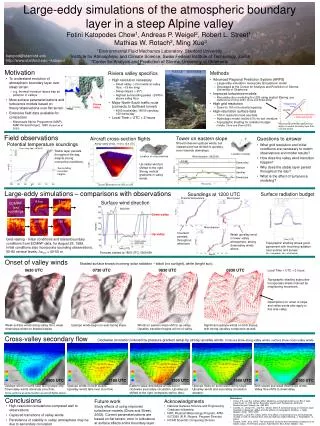

Aircraft cross-section flights
E N D
Presentation Transcript
Riviera Valley Downvalley Upslope Upvalley Downslope 0800 UTC 1100 UTC 1300 UTC 1600 UTC 2100 UTC Large-eddy simulations of the atmospheric boundary layer in a steep Alpine valley Fotini Katopodes Chow1, Andreas P. Weigel2, Robert L. Street1, Mathias W. Rotach2, Ming Xue3 1Environmental Fluid Mechanics Laboratory, Stanford University 2Institute for Atmospheric and Climate Science, Swiss Federal Institute of Technology, Zurich 3Center for Analysis and Prediction of Storms, University of Oklahoma katopod@stanford.edu http://www.stanford.edu/~katopod Motivation Methods Riviera valley specifics • To understand evolution of atmospheric boundary layer over steep terrain • e.g. thermal inversion layers trap air pollution in valleys • Most surface parameterizations and turbulence models based on theory/observations over flat terrain • Extensive field data available for comparison • Mesoscale Alpine Programme (MAP), MAP-Riviera Project, 1999 (Rotach et al. 2003) • Advanced Regional Prediction System (ARPS) • Large-eddy simulation mesoscale atmospheric model • Developed at the Center for Analysis and Prediction of Storms, University of Oklahoma • Improved turbulence models • Reconstruction modeling for LES using explicit filtering (see Gullbrand and Chow 2003, Chow and Street 2002) • High grid resolution • Down to 150 m horizontal spacing • High-resolution surface data • 100 m resolution land use data • Hydrologic model (WaSiM-ETH) for soil moisture • Topographic shading for radiation budget (Colette, Chow and Street 2003) • High resolution necessary • Small valley (~2 km wide at valley floor, ~15 km long) • Steep slopes (~35°) • Highest surrounding peaks ~2500m above valley floor • Major North-South traffic route (connects to Gotthard tunnel) • 4000 trucks/day, 14000 cars/day, 150 trains/day • Local Time = UTC + 2 hours Smagorinsky Log law Dynamic reconstruction + Near-wall model Reconstruction model captures log region in neutral boundary layer flow over flat terrain. Field observations Tower on eastern slope Should observe upslope winds, but instead wind has shifted to upvalley, even towards downslope. Questions to answer Aircraft cross-section flights Potential temperature soundings Along-valley winds, 11.6 to 12.4 UTC • What grid resolution and initial conditions are necessary to match observations and model results? • How does the valley wind transition happen? • Why does the stable layer persist throughout the day? • What is the effect of turbulence modeling? From valley floor, 08/25/99 Stable layer persists throughout the day, despite strong convective conditions. Location of tower Location of cross-sections Wind direction, 08/25/99 m ASL x 2 m agl x 13 m agl km ASL Up-valley wind jet shifted to the right. Strong vertical gradients in valley winds. degrees Surrounding mountain heights Time [UTC] position perpendicular to valley axis [m] K Large-eddy simulations– comparisons with observations Surface radiation budget Soundings at 1200 UTC Potential temperature Wind speed 9 km 3 km Surface wind direction ECMWF and soundings 08/25/99 km ASL km ASL Radiation flux [W/m2] Down-valley 1 km 350 m 150 m degrees m/s K Wind direction Inversion persists throughout afternoon Up-valley Weak upvalley wind in lower valley atmosphere, strong downvalley winds above Grid nesting - Initial conditions and lateral boundary conditions from ECMWF data, for August 25, 1999. Initial conditions also incorporate sounding observations. 50-60 vertical levels, Dzmin = 40-50 m Time [UTC] km ASL Topographic shading allows good agreement with incoming radiation near sunrise and sunset. (lw = longwave, sw = shortwave) Time [UTC] Forecast started at 1800 UTC, 08/24/99 degrees Onset of valley winds Shaded surface shows incoming solar radiation – black (no sunlight), white (bright sun). 0630 UTC 0730 UTC 0830 UTC 0930 UTC Local Time = UTC + 2 hours Topographic shading subroutine incorporates shade induced by neighboring mountains. Descriptions for onset of slope and valley winds also apply to this side valley. Weak surface winds along valley floor, weak downslope winds on shaded slopes. Upslope winds begin on east-facing slope. Winds on eastern slope shift to up-valley. Upvalley transition begins at foot of valley. Significant upslope winds on both slopes, with strong upvalley component as well. Cross-valley secondary flow Clockwise circulation induced by pressure gradient setup by strong upvalley winds. Contours show along-valley winds, vectors show cross-valley winds. m/s m/s m/s m/s Upslope wind on sunlit east-facing slope only. Downvalley winds dominate core flow. Upslope winds on both slopes. Upvalley winds take over core flow. Eastern slope downslope winds due to clockwise secondary circulation. Upvalley jet shifted to the right (compares well to obs.). Upslope flows on sunlit west-facing slope. Upvalley winds and secondary circulation weaken. Both slopes see weak downslope winds. Valley flow shifts to downvalley. Cross-sections at same location as aircraft flights above. Conclusions References • Chow, F.K. and R.L. Street. 2002. Modeling unresolved motions in LES of field-scale flows. In 15th Symp. Boundary Layers and Turbulence, American Meteorological Society, pp. 432-325. • Colette, A., Chow, F.K., and R.L. Street. 2003. A numerical study of inversion layer breakup in idealized valleys and the effects of topographic shading. J. Appl. Meteor. 42(9), 1255-1272. • Gullbrand, J. and F.K. Chow. 2003. The effect of numerical errors and turbulence models in LES of channel flow, with and without explicit filtering. J. Fluid Mech., in press. • Rotach, M.W., et al. 2003. The turbulence structure and exchange processes in an Alpine valley: The Riviera project. Submitted to Bull. Amer. Meteor. Soc. Acknowledgments • National Defense Science and Engineering Graduate fellowship • NSF, Physical Meteorology Program, ATM-0073395 (R.R. Rogers, Program Director) • NCAR Scientific Computing Division Future work Study effects of using improved turbulence models (Chow and Street, 2002). Current parameterizations are based on flat terrain; error in turbulence at surface affects entire boundary layer. • High-resolution simulations compared well to observations • Captured transitions of valley winds • Persistence of stability in valley atmosphere may be due to secondary circulation