Download
1 / 27
280 likes | 415 Views
This seminar by Larry Lamm covers key concepts in Particle Induced X-ray Emission (PIXE) data analysis, focusing on what the data can reveal and its inherent challenges. Key topics explore interactions between protons and atomic targets, the efficiency of detectors, and how to process and interpret output from detectors. The talk highlights the importance of understanding X-ray production, detector efficiency variations, and the process of fitting real data to theoretical models. Participants will gain insights into the complexities of data collection and analysis in PIXE studies.

E N D
PIXE: Data AnalysisWhat the data can(and cannot) tell us. Larry Lamm PIXE Seminar Winter 2008
Electron in orbit around the nucleus, In quantized energy level. electron nucleus proton Protons from the accelerator impinge upon the target. The atom spontaneously de-excites, releasing the excess energy in the form of an X-ray. Interaction with the passing proton excites the electron into a higher energy orbit.
Things to think about • Most (nearly all) of the X-rays produced are in directions such that they do not hit the detector!! (small solid angle).
Things to think about • Very rare – atom is mostly empty space – think of comets and our solar system, and how infrequently (thankfully!) a comet strikes Earth • Most (nearly all) of the X-rays produced are in a direction such that they do not hit the detector!! (small solid angle). • The detector is not perfectly efficient. Some X-rays that hit the detector will not be counted.
Things to think about • Detector efficiency varies with X-ray energy • Some elements more easily detected than others
There’s more • Pileup – when too many X-rays hit the detector at once • Escape peaks – when some of the energy from the X-ray is lost by the detector • Absorption – when X-rays are lost between the target and the detector by absorption (scattering) • Depth profiling in the sample
Glaze Pigment
There’s a lot going on here…. • Plenty of details to worry about… • How to measure the number of protons hitting the target? • Results will depend on this number • Difficult to measure in air (easy to do in vacuum) • Plunger target?
OK, but …. • So, a lot of details to worry about, but how can we proceed from here? • How do we get the data from the detector, and what information does it contain?
Output from detector • X-ray hits detector, produces lots of charge, which is collected by detector over a short time. Voltage Time
Conversion to digital (ADC) • The voltage signal from the detector must be digitized before it can be stored in the computer. The curve is integrated to find the area.
Conversion to digital (ADC) • The area under the curve is measured and is converted to a digital number. This number is a measure of the energy of the X-ray seen by the detector.
Histograms • The number from the ADC is collected and stored in a histogram – a collection of bins (we use 2048) scaled to match the energy spectrum of the X-rays we want to measure.
Histograms • As the ADC gives the number for the X-ray energy, the count in the appropriate bin is incremented, and over time the shape of the distribution begins to develop.
Typical Spectrum (INCO 625) • Here’s a histogram from a run on one of our standards, INCO 625. There are lots of peaks here.
INCO 625 • Same spectrum as previous, but in log scale to show low intensity peaks.
INCO 625 • The pileup, including double peaks, can clearly be seen. Also visible are some escape peaks. Escape Pileup
Fitting the data • A wealth of X-Ray data exists, see for example the X-Ray Data Booklet from LBNL (http://xdb.lbl.gov/)
X-Ray Energies • Tabulated in many places, including the X-Ray Data Booklet
X-Ray Intensities • Also tabulated are the relative intensities of these X-Rays, listed for each line of each element – at least in the X-Ray Data Booklet
Fitting Real Data to Theory • Start with something simple to illustrate • Consider a sample of pure silver (Ag) • We often use this to set up the detector
Ag X-Rays • Expand the region near the peaks for detail.
Ag X-Rays (Theory) • Calculate expected spectra based on data from the X-Ray Data Booklet.
Build the fit • Compare the theory to the data, with only a simple scale factor involved.
The scale factor • Getting this factor is the trick…. • GUPIX – a PIXE analysis software package from Guelph University, is the way most PIXE data is analyzed to determine the scale factor for the fits. • This scale factor can be used to determine abundances.
Fitting “by hand” • GUPIX is not magic… • We can do it all “by hand” – a lot of work, but very illustrative. That sounds hard! I can show you how…trust me!