Download

1 / 32
320 likes | 443 Views
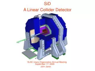
Instrumentation of the very Forward Region of a Linear Collider Detector. Wolfgang Lohmann. DESY (Zeuthen). Report from the FCAL workshop in Prague (April 16) Some results from SLAC (N. Graf and T Maruyama). The very Forward Calorimeter Collaboration Recent meeting in Prague, April 16.

E N D
Instrumentation of the very Forward Region of a Linear Collider Detector Wolfgang Lohmann DESY (Zeuthen) • Report from the FCAL workshop in Prague (April 16) • Some results from SLAC (N. Graf and T Maruyama) LC Workshop Paris
The very Forward Calorimeter Collaboration Recent meeting in Prague, April 16. see: PRC R&D 01/02
Functions of the very Forward Detectors • Measurement of the Luminosity (LumiCal) • Detection of Electrons and Photons at very low angle – extend hermiticity • Fast Beam Diagnostics (BeamCal) L* = 3m • Shielding of the inner Detector 300 cm VTX FTD IP BeamCal LumiCal
Measurement of the Luminosity Gauge Process: e+e- e+e- (g) Goal: 10-4 Precision (LEP: 3.4 exp.; 5.4 theor.) 10-4 10-4 Two Fermion Cross Sections at high Energy, Threshold Scans Physics Case: sZ for Giga-Z , • Technology: Si-W Sandwich Calorimeter Optimisation of shape and segmantation • MC Simulations • Alignment with Laser Beams • Close contacts to Theorists (Cracow, DESY)
Measurement of the Luminosity LumCal IP LumCal < 4 μm Requirements on Alignment and mechanical Precision (rough Estimate) < 0.7 mm Inner Radius of Cal.: < 1-4 μm Distance of Cals.: < 60 μm Radial beam position: < 0.7 mm
Measurement of the Luminosity Laser Alignment System • Simple CCD camera, • He-Ne red laser, • Laser translated in 50 mm steps Jagiellonian Univ. Cracow Photonics Group reconstruction of the laser spot (x,y) position on CCD camera
Measurement of the Luminosity R L e+e-e+e- (g) Simulations with BHWIDE 28 cm 15 cylinders * 24 sectors * 30 rings = 10800 cells 8 cm Rings 6.10m
Energy and Angular resolution Simulation: Bhwide(Bhabha)+CIRCE(Beamstrahlung)+beamspred Events selection: acceptance, energy balance, azimuthal and angular symmetry.
Stripped LumiCal acolinearity Qresolution Some systematics inQReconstruction !
Fast Beam Diagnostics (BeamCal) e+ e- • e+e-pairs from beamstrahlung are deflected into the LCAL • 15000 e+e- per BX 10 – 20 TeV • 10 MGy per year Rad. hard sensors GeV Technologies: Diamond-W Sandwich Scintillator crystals Gas ionisation chamber
Schematic views Heavy crystals W-Diamond sandwich sensor Space for electronics
Fast Beam Diagnostics (BeamCal) Observables detector: realistic segmentation, ideal resolution single parameter analysis, bunch by bunch resolution first radial moment first moment in 1/r thrust value total energy angular spread E(ring ≥ 4) / Etot (A + D) – (B + C) (A + B) – (C + D) E / N forward / backward calorimeter
Fast Beam Diagnostics (BeamCal) uncertainty. Beam Diag. nominal 1.5 2.1 ~ 10 % ~ 10 % Bunch width x Ave. Diff. 553 nm Bunch width y Ave. Diff. 5.0 nm Shintake Monitor 0.2 0.5 4.3 2.7 300 μm ~ 10 % ~ 10 % Bunch length z Ave. Diff. --- 0.7 Emittance in x Ave. Diff. 10.0 mm mrad ? ? ? ? 0.001 0.002 Emittance in y Ave. Diff. 0.03 mm mrad 6 0.4 Beam offset in x Beam offset in y 0 0 5 nm 0.1 nm --- 24 Horizontal waist shift Vertical waist shift 0 μm 360 μm None None detector: realistic segmentation, ideal resolution single parameter analysis, bunch by bunch resolution
Multi Parameter Analysis σx Δσx σy Δσy σz Δσz 0.3 % 0.4 % 3.4 % 9.5 % 1.4 % 0.8 % 1.5 % 0.9 % 0.3 % 0.4 % 3.5 % 11 % 0.9 % 1.0 % 11 % 24 % 5.7 % 24 % 1.6 % 1.9 % 1.8 % 1.1 % 16 % 27 % 3.2 % 2.1 %
σx = 650 nm σy = 3 nm First Look at Photons nominal setting (550 nm x 5 nm)
Detection of Electrons and Photons Efficiency to identify energetic electrons and photons (E > 200 GeV) Realistic beam simulation √s = 500 GeV Includes seismic motions, Delay of Beam Feedback System, Lumi Optimisation etc. Fake rate
High Energy Electron Detection in NLC LUMONN. Graf and T. Maruyama (SLAC) • Beampipe radius: IN 1 cm, OUT 2 cm • Detector: 50 layers of 0.2 cm W + 0.03 cm Si Zeuthen R- segmentation LUMON • Generate 330 bunches of pair backgrounds. • Pick 10 BX randomly and calculate average BG in each cell, <E>background • Pick one BX background and generate one high energy electron. • EBG + Eelectron - <E>background, in each cell • Apply electron finder. OUT IN 11 cm
High Energy Electron Detection 250 GeV Electron Pair Background BG 250 GeV e- Deposited Energy (arb. Units) Ebg + Eelectron - <Ebg> Si Layers
Electron finder 2 distribution Use first several layers as shield. • Use towers past layer 10 as seeds for a fixed-cone algorithm to cluster cells. - physical size of shower doesn’t change - simplifies geometry handling - single pass through the data • Cuts on cluster width and longitudinal shower 2. 250 GeV e- Background Cut at 450.
Efficiency (%) 100 90 80 70 60 50 Point 1 40 Point 2 Point 3 30 Point 4 20 Point 5 Point 6 10 0 50 100 150 200 250 Energy (GeV) Electron Detection Efficiency GeV 6 2 Y (cm) 3 5 4 1 X (cm)
Background Pileup What happens if we do not have single bunch time resolution? The detection efficiency does not degrade quickly, but the fake rake increases. Fake rate (all cluster energies): 1 bx 5% 2 20 3 40 4 47 Fakes are concentrated in hotspots, not uniform in phi. Expect rejection to improve with further study.
Sensor prototyping, Diamonds Different surface treatments : #1 – substrate side polished; 300 um #2 – cut substrate; 200 um #3 – growth side polished; 300 um #4 – both sides polished; 300 um Diamond; Size: 12x12 mm 2 Metallisation: 10 nm Ti + 400nm Au Current (I) dependence on the voltage (V) Ohmic behavior for ‘ramping up/down’, hysteresis Charge collection distance is saturated to 60 mm at ~300V
Sensor prototyping, Diamonds Charge Collection distance vs. dose #2 – cut substrate; 200 um #1 – substrate side polished; 300 um
Preamplifier Characteristics Oscillograms of Tetrod-BJT Amplifier Preamp output 20ns/div Shaper output 20ns/div
Sensor prototyping, Crystals Light Yield from direct coupling Plastic scintilator and using a fibre Study with heavy crystals (Cerenkov light) is going on ~ 15 %
Sensor prototyping, C3F8 Gas Ionisation Chamber Pads for charge collection Beam Test,e- beam, 10-40 GeV (IHEP) Pressure vessel
Offers for GaAs LPI group Lebedev Physical Institute, Moscow IHEP, Protvino NCPHEP, Minsk SIPT, Tomsk ICBP, Puschino
Summary • MC Simulations to optimise the Design of the forward calorimeters are progressing • Different Detector Technologies for BeamCal are under study • BeamCal has a great potential for fast beam diagnostics • Tests with Sensor Prototypes and preamplifier have been started • After about one year we will present a Design • The goal is to start after with the construction and test of a prototype
Charge collection distance measurements Qmeas. = Qcreated x ccd / L ADC Sr90 PA delay diamond Scint. discr & PM1 Gate discr PM2 Using electrons from a Sr90 source (mips)
Charge collection distance measurements The sensors are not irradiated Upper curve is ramping up HV, Lower ramping down. Charge collection distance is saturated to 50 mm at ~300V
Sensor prototyping and lab tests Current (I) dependence on the voltage (V) Ohmic behavior for ‘ramping up/down’, hysteresis Resistance in the order of 100 TOhm Current decays with time After 24 h nearly 1/2
Detection of Electrons and Photons • essential parameters: Small Molière radius High granularity Longitudinal segmentation • Two photon event rejection e+e- e+e-m+m- (Severe background for particle searches) • Electromagnetic fakes 1% from physics 2% from fluctuations