Models for Parallel Computers
Models for Parallel Computers. Goals of a machine model accurately reflect constraints of existing machines broad applicability with respect to existing and future machines allows accurate prediction of performance Models being discussed PRAM BSP LogP.

Models for Parallel Computers
E N D
Presentation Transcript
Models for Parallel Computers • Goals of a machine model • accurately reflect constraints of existing machines • broad applicability with respect to existing and future machines • allows accurate prediction of performance • Models being discussed • PRAM • BSP • LogP
Parallel Random Access Machine (PRAM) • PRAM • S. Fortune, J. Wyllie, Parallelism in Random Access Machines, 10th ACM Symposium on Theory of Computing, pp. 114-118, 1978 • Abstraction of a synchronized MIMD computer with shared memory • Definition of a n-PRAM • It is a parallel register machine with n processors P0, ..., Pn-1 with a shared memory. • In each step, each processor can work as a separate register machine or can access a cell of the shared memory. • The processors are working synchronously, one step takes unit time.
PRAM (2): Example • Task • Given are n variables X0, ..., Xn-1{0,1}. • Compute function ORn with ORn(X0,...,Xn-1)=1 iff i{0,...,n-1} with Xi=1 • Solution 1: • Use n-PRAM • Calculate on a tree network in which each inner node performs the operation OR2 with data sent from its sons. The root gets the result. • This solution has runtime O(log n).
PRAM (3): Example • Solution 2: • Use a n-PRAM, let processor Pi access variable Xi. for all processors Pi pardo if Xi=1 then Result :=1 od • This solution has constant runtime.
PRAM (4) • Different PRAM models: • Exclusive Read Exclusive Write (EREW): It is not possible to read or write a memory cell simultaneously with several processors. • Concurrent Read Exclusive Write (CREW): It is only possible to read a cell simultaneously. • Concurrent Read Concurrent Write (CRCW): Processors can read and write a cell simultaneously. Concurrent write forces to define which one of the concurrent processors will win. • Arbitrary: One processor wins, but it is not known in advance which one wins. • Common: All processors must write identical data. • Priority: The processor with the largest or lowest index wins.
PRAM(5) • A CRCW PRAM can be simulated on a EREW PRAM • Delay O(log n), e.g. 256 processors can be simulated with 8c where c is a constant factor - the simulation overhead.
PRAM (6) • The PRAM model favors maximal parallelism. • It does not take aspects of real machines into account. Machines do not provide: • Unit time communication cost, no contention • Synchronous execution and therefore explicit synchronization is required. • Hardware implementation of a PRAM at Fachbereich 14, Universität des Saarlandes (Prof. Wolfgang Paul) • Fork language (Christoph Kessler, Universität Trier)
Bulk-Synchronous Parallel Model (BSP) • Definition BSP machine • It consists of processors with local memory connected by a communication network. • It performs a sequence of supersteps consisting of three phases: • Local computation phase: • asynchronous operations • extract messages from an input buffer • insert messages into an output buffer • Communication phase: • messages are transferred from output buffer to destination input buffer • Barrier synchronization concludes superstep and makes moved data available in the local memories.
Superstep Processors • Execution time of a superstep w + g h + l • w is the maximum number of local operations performed by any processor • h is the maximum number of messages sent or received by any processor (h-relation) • g reflects the bandwidth measured in time units per message • l upper bound of global synchronization time Synchronization
Other Cost Functions of a Superstep • Overlapping communication and computation MAX(w, hg) + L • Taking into account the sequence of sending and receiving messages (hin + hout) g • The cost model does not take into account: • splitting cost in startup and transfer cost • locality: mapping the processes in the right way onto the machine will reduce contention and communication distance. • L.G. Valiant: A Bridging Model for Parallel Computation, Communications of the ACM, Vol. 33, No. 8, pp. 103-111, 1990 • users.comlab.ox.ac.uk/bill.mccoll/oparl.html
Broadcast • Summary: Broadcasting • When N is small ( i.e., N<l/(pg-2g) use the one-stage broadcast • The two-stage broadcast is always better than the tree broadcast when p>4 • Most communication libraries still implement broadcast by the tree based technique • Good BSP design = Balanced design
BSP • The BSP model describes a special but realistic computational structure • It allows to study the influence of synchronization and communication. • It allows for asynchronous computation.
LogP • LogP model takes into account latency, overhead and bandwidth of the communication. • David Culler, A Practical Model of Parallel Computation, Communications of the ACM, Vol. 39, No.11, November 1996
LogP • A parallel computer is described in the LogP model by the following parameters: • L: An upper bound on the latency, or delay, incurred in communicating a message containing a word from its source node to its target node. • o: The overhead, defined as the time that a processor is engaged in the transmission or reception of each message. During this time the processor cannot perform other operations. • g: The gap, defined as the minimum time interval between consecutive message transmissions or receptions. The reciprocal of g corresponds to the available per-processor bandwidth • P: The number of processor/memory modules.
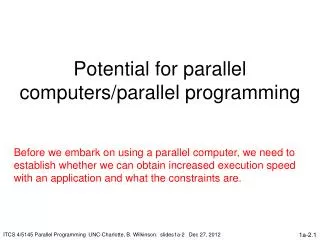
LogP (2) P P P M M M • The latency experienced by any message is unpredictable, but it is bound by L. • The network is treated as a pipeline of length L with initiation rate g and a processor overhead of o on each end. • The capacity of the network is finite. No more than L/g messages can be in transit from a processor at any time. g (gap) o (overhead) o L (latency) Interconnection Network
LogP Implementation of Broadcast P=8, L=6, g=4, o=2 Total execution time: 24
LogP (3) • The LogP model takes into account latency and overhead for message transmission. • The technique of multithreading is often suggested as a way of masking latency. In practice this technique is limited by the available communication bandwidth. This is taken into account by the finite network capacity. • It does encourage • techniques optimizing the data placement to reduce amount and frequency of communication. • latency hiding techniques. • It does not model • local operations • explicit synchronization operations • details of the interconnection topology
Summary • Models highlight different aspects of the machine. • PRAM: parallelism • BSP: coarse communication model, special programming structure • LogP: detailed communication model