ALGORITHM TYPES
Learn about the Greedy approach for scheduling problems to minimize the sum of finish times, with examples and strategies. Compare to other algorithms like Dynamic Programming and Divide and Conquer. Ideal for understanding optimization in job scheduling scenarios.

ALGORITHM TYPES
E N D
Presentation Transcript
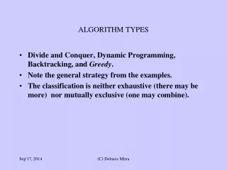
ALGORITHM TYPES Divide and Conquer, Dynamic Programming, Backtracking, and Greedy. Note the general strategy from the examples. The classification is neither exhaustive (there may be more) nor mutually exclusive (one may combine). (C) Debasis Mitra
GREEDY Approach: Scheduling problem – Minimize Sum-of-FTProblem 1 Input: set of (job-id, duration) pairs, e.g. (j1, 15), (j2, 8), (j3, 3), (j4, 10) Objective function: Sum over Finish Time of all jobs: in above order, it is 15+23+26+36=100 Output: Best schedule, for least value of Obj. Func. How many possibilities to try? (j1, j2, j3, j4), (j1, j2, j4, j3), (j1, j3, j2, j4), … 4 possibilities for the first position, then 3 for second, 2 for the third, and the only left job goes to the last => 4.3.2.1 = 4! n! , for n jobs, if you try all possibilities (C) Debasis Mitra
GREEDY Approach: Scheduling problem – Minimize Sum-of-FT Input: list of (job-id, duration) pairs, e.g. (j1, 15), (j2, 8), (j3, 3), (j4, 10) Objective function: Sum over Finish Time of all jobs: in above order, it is 15+23+26+36=100 Output: Best schedule, for least value of Obj. Func. What do you think the best order should be? Note: durations of tasks are getting added multiple times: 15 + (15+8) + ((15+8) + 3) + (((15+8) +3) +10) = 15x4 + 8x3 +3x2 +1x10 Yes, the best order is shortest-job-first! Greedy schedule: j3, j2, j4, j1. Aggregate FT=3+11+21+36=71 [Let the lower values get added more times: shortest job first] This happens to be the best schedule: Optimum Complexity: Sort first: O(n log n), then place: (n), Total: O(n log n) (C) Debasis Mitra
MULTI-PROCESSOR SCHEDULING (Aggregate FT)Problem 2 Input: set of (job-id, duration), & number of processors e.g. {(j2, 5), (j1, 3), (j5, 11), (j3, 6), (j4, 10), (j8, 18), (j6, 14), (j7, 15), (j9, 20)}, & 3 proc Objective Fn.: Aggregate FT (AFT) Output: Least AFT Greedy Strategy: Pre-sort jobs from low to high Then, assign ordered jobs over the processors one by one Sort: (j1, 3), (j2, 5), (j3, 6), (j4, 10), (j5, 11), (j6, 14), (j7, 15), (j8, 18), (j9, 20) // O (n log n) Schedule next job on an earliest available processor Complexity for assignment: O(n m) for m processors, dominates over O(n log n) Do you agree, O(n, m)? (C) Debasis Mitra
MULTI-PROCESSOR SCHEDULING (Aggregate FT)Problem 2 Input: set of (job-id, duration), & number of processors e.g. {(j2, 5), (j1, 3), (j5, 11), (j3, 6), (j4, 10), (j8, 18), (j6, 14), (j7, 15), (j9, 20)}, & 3 proc Sort: {(j1, 3), (j2, 5), (j3, 6), (j4, 10), (j5, 11), (j6, 14), (j7, 15), (j8, 18), (j9, 20)}, 3 Schedule next job on an earliest available processor Proc 1: Proc 2: Proc 3: Aggregate-FT = 3+13+28+5+… = 152 For each job, assign just the next processor sequentially, cycling back to 1 after m, do not need to seek for next available processor: time-complexity of assignment = O(n), total: O(n log n) j13 J43+10 J713+15 j25 J55+11 J816+18 j36 J66+14 J920+20 (C) Debasis Mitra
Input: Set of (job, duration) pairs, and #processors Objective Fn.: Last Finish Time over all processors Output: Best schedule Strategy? Greedy Strategy: Sort jobs in reverse order, Then, assign next job on the earliest available processor (j3, 6), (j1, 3), (j2, 5), (j4, 10), (j6, 14), (j5, 11), (j8, 18), (j7, 15), (j9, 20): 3 processor Reverse sort- (j9, 20), (j8, 18), (j7, 15), (j6, 14), (j5, 11), (j4, 10), (j3, 6), (j2, 5), (j1, 3) MULTI-PROCESSOR SCHEDULING (Last FT)Problem 3 (C) Debasis Mitra
Input: (j3, 6), (j1, 3), (j2, 5), (j4, 10), (j6, 14), (j5, 11), (j8, 18), (j7, 15), (j9, 20): 3 processor Reverse sort: (j9, 20), (j8, 18), (j7, 15), (j6, 14), (j5, 11), (j4, 10), (j3, 6), (j2, 5), (j1, 3) Schedule next job on an earliest available processor Proc 1: Proc 2: Proc 3: MULTI-PROCESSOR SCHEDULING (Last FT) J420+10 j920 J130+3 j818 J518+11 J329+6 j715 J615+14 J229+5 Last-Finish-Time = 35 Complexities? (C) Debasis Mitra
Input: Set of (job, duration) pairs, and #processors Output: Best schedule Objective Fn.: Last Finish Time over all jobs Greedy Strategy: Sort jobs in reverse order, Then, assign next job on the earliest available processor Time-complexity sort: O(n log n) place: naïve: (nM), with heap over processors: O(n log m) O(log m) using HEAP, total O(n logn + n logm) or O(max{n logn, m logm}), for n>>m the first term dominates Space complexity? Space complexity: O(n), for all jobs MULTI-PROCESSOR SCHEDULING (Last FT) (C) Debasis Mitra
(j3, 6), (j1, 3), (j2, 5), (j4, 10), (j6, 14), (j5, 11), (j8, 18), (j7, 15), (j9, 20): 3 processor GreedySchedule: Proc 1: j9 - 20, j4 - 30, j1 - 33. Proc 2: j8 - 18, j5 - 29, j3 - 35, Proc 3: j7 - 15, j6 - 29, j2 - 34, Greedy Last-FT = 35. OptimalSchedule: Proc1: j2, j5, j8: 5+11+18=34 Proc 2: j6, j9: 14+20=34 Proc 3: j1, j3, j4, j7 : 3+6+10+15=34 OptimumLast-FT = 34. Greedy algorithm is NOT optimal algorithm here, but the relative error ≤ [1/3 - 1/(3m)], for m processors Relative error = (greedyLFT –optimalLFT) / optimalLFT An NP-complete problem, greedy algorithm is polynomial providing approximate solution MULTI-PROCESSOR SCHEDULING (Last FT) (C) Debasis Mitra
HUFFMAN ENCODINGProblem 4 Problem: formulate a (binary) coding of keys (e.g. character) for a text, Input: given a set of (character, frequency) pairs (as appears in the text) Objective Function: total number of bits in the text Output: Variable bit-size encoding, s.t. the objective function is minimum Output Encoding: A binary tree with the characters on leaves (each edge indicating 0 or 1) 0 space (13) e (15) i (12) a (10) t (4) newline (1) s (3) (C) Debasis Mitra
Total bits in the text for above encoding: (a, code: 001, freq=10, total=3x10=30 bits), (e, code: 01, f=15, 2x15=30 bits), (i, code: 10, f=12, 24 bits), (s, code: 00000, f=3, 15 bits), (t, code: 0001, f=4, 16 bits), (space, code: 11, f=13, 26 bits), (newline, code: 00001, f=1, 5 bits), Total bits=146 bits HUFFMAN ENCODINGProblem 4 Input: (a, freq=10), (e, 15), (i, 12), (s, 3), (t, 4), (space, 13), (newline, 1) 1 0 0 An arbitrary encoding space (13) e (15) i (12) a (10) t (4) newline (1) s (3) (C) Debasis Mitra
Start from a forest of all nodes (alphabets) with their frequencies being their weights At every iteration, form a binary tree using the two smallest (lowest aggregate frequency) available trees in a forest Declare the resulting tree’s frequency as the aggregate of its leaves’ frequency. When the final single binary-tree is formed return that as the output (for using that tree for encoding the text) HUFFMAN ENCODING: Greedy Algorithm (C) Debasis Mitra
HUFFMAN ENCODING: Greedy Algorithm Source: Weiss, pg 390 (C) Debasis Mitra
HUFFMAN ENCODING: Greedy Algorithm Source: Weiss, pg 390 (C) Debasis Mitra
HUFFMAN ENCODING: Greedy Algorithm Source: Weiss, pg 391 (C) Debasis Mitra
HUFFMAN ENCODING: greedy alg.’s complexityProblem 4 First, initialize a min-heap (priority queue) for n nodes’ frequencies: O(n) Pick 2 best (minimum) trees: 2(log n) Insert 1 tree in the heap: O(log n) Do that for an order of n times: O(n log n) Total: O(n log n) Heap is needed, because the sorted list is not static Otherwise, one needs to do repeated sorting in every iteration (C) Debasis Mitra
RATIONAL KNAPSACKProblem 5 Input: a set of objects with (Weight, Profit), and a Knapsack of limited weight capacity (M) Output: find a subset of objects to maximize profit, partial objects (broken) are allowed, subject to total wt <=M Greedy Algorithm: Put objects in the KS in a non-increasing (high to low) order of profit density (profit/weight). Break the object which does not fit in the KS otherwise – this will be last object to be in the knapsack. Optimal, polynomial algorithm O(N log N) for N objects - from sorting. (C) Debasis Mitra
RATIONAL KNAPSACKProblem 5 Greedy Algorithm: Put objects in the KS in a non-increasing (high to low) order of profit density (profit/weight). Break the object which does not fit in the KS otherwise – this will be last object to be in the knapsack. Example: (O1, 4, 12), (O2, 5, 20), (O3, 10, 10), (O4, 12, 6); M=14. Solution: 1. Sort={(O2, 20/5), (O1, 12/4), (O3, 10/10), (O4, 6/12)} 2. KS= {O2, O1, ½ of O3}, Wt=4+5+ ½ of 10=14, same as M Profit=12+20+ ½ 10 = 37 Optimal profit – cannot make any better polynomial algorithm O(N log N) for N objects - from sorting. [0-1 KS problem: cannot break any object: NP-complete, Greedy Algorithm is no longer optimal] (C) Debasis Mitra
APPROXIMATE BIN PACKING Problem: fill in objects each of size<= 1, in minimum number of bins (optimal) each of size=1 (NP-complete). Example: 0.2, 0.5, 0.4, 0.7, 0.1, 0.3, 0.8. Solution: B1: 0.2+0.8, B2: 0.3+0.7, B3: 0.1+0.4+0.5. All bins are full, so must be optimal solution (note: optimal solution need not have all bins full). Online problem: do not have access to the full set: incremental; Offline problem: can order the set before starting. (C) Debasis Mitra
ONLINE BIN PACKING Theorem 1: No online algorithm can do better than 4/3 of the optimal #bins, for any given input set. Proof. (by contradiction: we will use a particular input set, on which our online algorithm A presumably violates the Theorem) Consider input of M items of size 1/2 - k, followed by M items of size 1/2 + k, for 0<k<0.01 [Optimum #bin should be M for them.] Suppose alg A can do better than 4/3, and it packs first M items in b bins, which optimally needs M/2 bins. So, by assumption of violation of Thm, b/(M/2)<4/3, or b/M<2/3 [fact 0] (C) Debasis Mitra
ONLINE BIN PACKING • Each bin has either 1 or 2 items • Say, the first b bins containing x items, • So, x is at most or 2b items • So, left out items are at least or (2M-x) in number [fact 1] • When A finishes with all 2M items, all 2-item bins are within the first b bins, • So, all of the bins after first b bins are 1-item bins [fact 2] • fact 1 plus fact 2: after first b bins A uses at least or (2M-x) number of bins or BA (b + (2M - 2b)) = 2M - b. (C) Debasis Mitra
ONLINE BIN PACKING - So, the total number of bins used by A (say, BA) is at least or, BA (b + (2M - 2b)) = 2M - b. - Optimal needed are M bins. - So, (2M-b)/M < (BA /M) 4/3 (by assumption), or, b/M>2/3 [fact 4] - CONTRADICTION between fact 0 and fact 4 => A can never do better than 4/3 for this input. (C) Debasis Mitra
NEXT-FIT ONLINE BIN-PACKING If the currentitem fits in the currentbin put it there, otherwise move on to the next bin. Linear time with respect to #items - O(n), for n items. Example: Weiss Fig 10.21, page 364. Thm 2: Suppose, M optimum number of bins are needed for an input. Next-fit never needs more than 2M bins. Proof: Content(Bj) + Content(Bj+1) >1, So, Wastage(Bj) + Wastage(Bj+1)<2-1, Average wastage<0.5, less than half space is wasted, so, should not need more than 2M bins. (C) Debasis Mitra
FIRST-FIT ONLINE BIN-PACKING Scan the existing bins, starting from the first bin, to find the place for the next item, if none exists create a new bin. O(N2) naïve, O(NlogN) possible, for N items. Obviously cannot need more than 2M bins! Wastes less than Next-fit. Thm 3: Never needs more than Ceiling(1.7M). Proof: too complicated. For random (Gaussian) input sequence, it takes 2% more than optimal, observed empirically. Great! (C) Debasis Mitra
BEST-FIT ONLINE BIN-PACKING Scan to find the tightest spot for each item (reduce wastage even further than the previous algorithms), if none exists create a new bin. Does not improve over First-Fit in worst case in optimality, but does not take more worst-case time either! Easy to code. (C) Debasis Mitra
OFFLINE BIN-PACKING Create a non-increasing order (larger to smaller) of items first and then apply some of the same algorithms as before. GOODNESS of FIRST-FIT NON-INCREASING ALGORITHM: Lemma 1: If M is optimal #of bins, then all items put by the First-fit in the “extra” (M+1-th bin onwards) bins would be of size 1/3 (in other words, all items of size>1/3, and possibly some items of size 1/3 go into the first M bins). Proof of Lemma 1. (by contradiction) Suppose the lemma is not true and the first object that is being put in the M+1-th bin as the Algorithm is running, is say, si, is of size>1/3. Note, none of the first M bins can have more than 2 objects (size of each>1/3). So, they have only one or two objects per bin. (C) Debasis Mitra
Proof of Lemma 1 continued. We will prove that the first j bins (0 jM) should have exactly 1 item each, and next M-j bins have 2 items each (i.e., 1 and 2 item-bins do not mix in the sequence of bins) at the time si is being introduced. Suppose contrary to this there is a mix up of sizes and bin# B_x has two items and B_y has 1 item, for 1x<yM. The two items from bottom in B_x, say, x1 and x2; it must be x1y1, where y1 is the only item in B_y At the time of entering si, we must have {x1, x2, y1} si, because si is picked up after all the three. So, x1+ x2 y1 + si. Hence, if x1 and x2 can go in one bin, then y1 and si also can go in one bin. Thus, first-fit would put si in By, and not in the M+1-th bin. This negates our assumption that single occupied bins could mix with doubly occupied bins in the sequence of bins (over the first M bins) at the moment M+1-th bin is created. OFFLINE BIN-PACKING (C) Debasis Mitra
Proof of Lemma 1 continued: Now, in an optimal fitthat needs exactly M bins: si cannot go into first j-bins (1 item-bins), because if it were feasible there is no reason why First-fit would not do that (such a bin would be a 2-item bin within the 1-item bin set). Similarly, if si could go into one of the next (M-j) bins (irrespective of any algorithm), that would mean redistributing 2(M-j)+1 items in (M-j) bins. Then one of those bins would have 3 items in it, where each item>1/3 (because si>1/3). So, si cannot fit in any of those M bins by any algorithm, if it is >1/3. Also note that if si does not go into those first j bins none of objects in the subsequent (M-j) bins would go either, i.e., you cannot redistribute all the objects up to si in the first M bins, or you need more than M bins optimally. This contradicts the assumption that the optimal #bin is M. Restating: either si 1/3, or if si goes into (M+1)-th bin then optimal number of bins could not be M. In other words, all items of size >1/3 goes into M or lesser number of bins, when M is the optimal #of bins for the given set. End of Proof of Lemma 1. OFFLINE BIN-PACKING (C) Debasis Mitra
Lemma 2: The #of objects left out after M bins are filled (i.e., the ones that go into the extra bins, M+1-th bin onwards) are at most M. [This is a static picture after First Fit finished working] Proof of Lemma 2. On the contrary, suppose there are M or more objects left. [Note that each of them are <1/3 because they were picked up after si from the Lemma 1 proof.] Note, j=1Nsj M, since M is optimum #bins, where N is #items. Say, each bin Bj of the first M bins has items of total weight Wj in each bin, and xk represent the items in the extra bins ((M+1)-th bin onwards): x1, …, xM, … OFFLINE BIN-PACKING (C) Debasis Mitra
OFFLINE BIN-PACKING • i=1N si j=1M Wj + k=1Mxk (the first term sums over bins, & the second term over items) = j=1M (Wj + xj) • But i=1N si M, • or, j=1M (Wj + xj) i=1N si M. • So, Wj+xj 1 • But, Wj+xj > 1, otherwise xj (or one of the xi’s) would go into the bin containing Wj, by First-fit algorithm. • Therefore, we have i=1Nsi > M. A contradiction. End of Proof of Lemma 2. (C) Debasis Mitra
Theorem: If M is optimum #bins, then First-fit-offline will not take more than M + (1/3)M #bins. Proof of Theorem10.4. #items in “extra” bins is M. They are of size 1/3. So, 3 or more items per those “extra” bins. Hence #extra bins itself (1/3)M. # of non-extra (initial) bins = M. Total #bins M + (1/3)M End of proof. OFFLINE BIN-PACKING (C) Debasis Mitra