Index Compression
Index Compression. Adapted from Lectures by Prabhakar Raghavan (Yahoo and Stanford) and Christopher Manning (Stanford). Last lecture – index construction. Key step in indexing – sort This sort was implemented by exploiting disk-based sorting Fewer disk seeks Hierarchical merge of blocks

Index Compression
E N D
Presentation Transcript
Index Compression Adapted from Lectures by Prabhakar Raghavan (Yahoo and Stanford) and Christopher Manning (Stanford) L07IndexCompression
Last lecture – index construction • Key step in indexing – sort • This sort was implemented by exploiting disk-based sorting • Fewer disk seeks • Hierarchical merge of blocks • Distributed indexing using MapReduce • Running example of document collection: RCV1 L07IndexCompression
Today • Collection statistics in more detail (RCV1) • Dictionary compression • Postings compression L07IndexCompression
Recall Reuters RCV1 • symbol statistic value • N documents 800,000 • L avg. # tokens per doc 200 • M terms (= word types) ~400,000 • avg. # bytes per token 6 (incl. spaces/punct.) • avg. # bytes per token 4.5 (without spaces/punct.) • avg. # bytes per term 7.5 • non-positional postings 100,000,000 L07IndexCompression
Why compression? • Keep more stuff in memory (increases speed, caching effect) • enables deployment on smaller/mobile devices • Increase data transfer from disk to memory • [read compressed data and decompress] is faster than [read uncompressed data] • Premise: Decompression algorithms are fast • True of the decompression algorithms we use L07IndexCompression
Compression in inverted indexes • First, we will consider space for dictionary • Make it small enough to keep in main memory • Then the postings • Reduce disk space needed, decrease time to read from disk • Large search engines keep a significant part of postings in memory • (Each postings entry is a docID) L07IndexCompression
Index parameters vs. what we index (details Table 5.1 p80) Exercise: give intuitions for all the ‘0’ entries. Why do some zero entries correspond to big deltas in other columns?
Lossless vs. lossy compression • Lossless compression: All information is preserved. • What we mostly do in IR. • Lossy compression: Discard some information • Several of the preprocessing steps can be viewed as lossy compression: case folding, stop words, stemming, number elimination. • Chap/Lecture 7: Prune postings entries that are unlikely to turn up in the top k list for any query. • Almost no loss of quality for top k list. L07IndexCompression
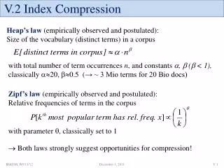
Vocabulary vs. collection size • Heaps’ Law: M = kTb • M is the size of the vocabulary, T is the number of tokens in the collection. • Typical values: 30 ≤ k ≤ 100 and b ≈ 0.5. • In a log-log plot of vocabulary vs. T, Heaps’ law is a line. L07IndexCompression
Heaps’ Law Fig 5.1 p81 For RCV1, the dashed line log10M = 0.49 log10T + 1.64 is the best least squares fit. Thus, M = 101.64T0.49so k = 101.64 ≈ 44 and b = 0.49. L07IndexCompression
Zipf’s law • We also study the relative frequencies of terms. • In natural language, there are a few very frequent terms and very many rare terms. • Zipf’s law: The ith most frequent term has frequency proportional to 1/i . • cfi ∝ 1/i = c/i where c is a normalizing constant • cfi is collection frequency: the number of occurrences of the term ti in the collection. L07IndexCompression
Zipf consequences • If the most frequent term (the) occurs cf1 times • then the second most frequent term (of) occurs cf1/2 times • the third most frequent term (and) occurs cf1/3 times … • Equivalent: cfi = c/i where c is a normalizing factor, so • log cfi = log c - log i • Linear relationship between log cfi and log i L07IndexCompression
Compression • First, we will consider space for dictionary and postings • Basic Boolean index only • No study of positional indexes, etc. • We will devise compression schemes L07IndexCompression
Dictionary Compression L07IndexCompression
Why compress the dictionary • Must keep in memory • Search begins with the dictionary • Memory footprint competition • Embedded/mobile devices L07IndexCompression
Dictionary storage - first cut • Array of fixed-width entries • ~400,000 terms; 28 bytes/term = 11.2 MB. Dictionary search structure 20 bytes 4 bytes each L07IndexCompression
Fixed-width terms are wasteful • Most of the bytes in the Term column are wasted – we allot 20 bytes for 1 letter terms. • And we still can’t handle supercalifragilisticexpialidocious. • Written English averages ~4.5 characters/word. • Ave. dictionary word in English: ~8 characters • How do we use ~8 characters per dictionary term? • Short words dominate token counts but not token type (term) average. L07IndexCompression
Compressing the term list: Dictionary-as-a-String • Store dictionary as a (long) string of characters: • Pointer to next word shows end of current word • Hope to save up to 60% of dictionary space. ….systilesyzygeticsyzygialsyzygyszaibelyiteszczecinszomo…. Total string length = 400K x 8B = 3.2MB Pointers resolve 3.2M positions: log23.2M = 22bits = 3bytes L07IndexCompression
Space for dictionary as a string • 4 bytes per term for Freq. • 4 bytes per term for pointer to Postings. • 3 bytes per term pointer • Avg. 8 bytes per term in term string • 400K terms x 19 7.6 MB (against 11.2MB for fixed width) Now avg. 11 bytes/term, not 20. L07IndexCompression
Blocking • Store pointers to every kth term string. • Example below: k=4. • Need to store term lengths (1 extra byte) ….7systile9syzygetic8syzygial6syzygy11szaibelyite8szczecin9szomo…. Save 9 bytes on 3 pointers. Lose 4 bytes on term lengths.
Net • Where we used 3 bytes/pointer without blocking • 3 x 4 = 12 bytes for k=4 pointers, now we use 3+4=7 bytes for 4 pointers. Shaved another ~0.5MB; can save more with larger k. Why not go with larger k? L07IndexCompression
Exercise • Estimate the space usage (and savings compared to 7.6 MB) with blocking, for block sizes of k = 4, 8 and 16. • For k = 8. • For every block of 8, need to store extra 8 bytes for length • For every block of 8, can save 7 * 3 bytes for term pointer • Saving (+8 – 21)/8 * 400K = 0.65 MB L07IndexCompression
Dictionary search without blocking Assuming each dictionary term equally likely in query (not really so in practice!), average number of comparisons = (1+2∙2+4∙3+4)/8 ~2.6 L07IndexCompression
Dictionary search with blocking • Binary search down to 4-term block; • Then linear search through terms in block. • Blocks of 4 (binary tree), avg. = (1+2∙2+2∙3+2∙4+5)/8 = 3 compares L07IndexCompression
Exercise • Estimate the impact on search performance (and slowdown compared to k=1) with blocking, for block sizes of k = 4, 8 and 16. • logarithmic search time to get to get to (n/k) “leaves” • linear time proportional to k/2 for subsequent search through the “leaves” • closed-form solution not obvious L07IndexCompression
Front coding • Front-coding: • Sorted words commonly have long common prefix – store differences only • (for last k-1 in a block of k) 8automata8automate9automatic10automation 8automat*a1e2ic3ion Extra length beyond automat. Encodes automat Begins to resemble general string compression.
RCV1 dictionary compression L07IndexCompression
Postings compression L07IndexCompression
Postings compression • The postings file is much larger than the dictionary, by a factor of at least 10. • Key desideratum: store each posting compactly. • A posting for our purposes is a docID. • For Reuters (800,000 documents), we would use 32 bits per docID when using 4-byte integers. • Alternatively, we can use log2 800,000 ≈ 20 bits per docID. • Our goal: use a lot less than 20 bits per docID. L07IndexCompression
Postings: two conflicting forces • A term like arachnocentric occurs in maybe one doc out of a million – we would like to store this posting using log2 1M ~ 20 bits. • A term like the occurs in virtually every doc, so 20 bits/posting is too expensive. • Prefer 0/1 bitmap vector in this case L07IndexCompression
Postings file entry • We store the list of docs containing a term in increasing order of docID. • computer: 33,47,154,159,202 … • Consequence: it suffices to store gaps. • 33,14,107,5,43 … • Hope: most gaps can be encoded/stored with far fewer than 20 bits. L07IndexCompression
Three postings entries L07IndexCompression
Variable length encoding • Aim: • For arachnocentric, we will use ~20 bits/gap entry. • For the, we will use ~1 bit/gap entry. • If the average gap for a term is G, we want to use ~log2G bits/gap entry. • Key challenge: encode every integer (gap) with ~ as few bits as needed for that integer. • Variable length codes achieve this by using short codes for small numbers L07IndexCompression
Variable Byte (VB) codes • For a gap value G, use close to the fewest bytes needed to hold log2 G bits • Begin with one byte to store G and dedicate 1 bit in it to be a continuation bit c • If G ≤127, binary-encode it in the 7 available bits and set c =1 • Else encode G’s lower-order 7 bits and then use additional bytes to encode the higher order bits using the same algorithm • At the end set the continuation bit of the last byte to 1 (c =1) and of the other bytes to 0 (c =0).
Example Postings stored as the byte concatenation 00000110 10111000 10000101 00001101 00001100 10110001 Key property: VB-encoded postings are uniquely prefix-decodable. For a small gap (5), VB uses a whole byte.
Other variable codes • Instead of bytes, we can also use a different “unit of alignment”: 32 bits (words), 16 bits, 4 bits (nibbles) etc. • Variable byte alignment wastes space if you have many small gaps – nibbles do better in such cases. L07IndexCompression
Gamma codes • Can compress better with bit-level codes • The Gamma code is the best known of these. • Represent a gap G as a pair length and offset • offset is G in binary, with the leading bit cut off • For example 13 → 1101 → 101 • length is the length of offset • For 13 (offset 101), this is 3. • Encode length in unary code: 1110. • Gamma code of 13 is the concatenation of length and offset: 1110101 L07IndexCompression
Gamma code examples L07IndexCompression
Exercise • Given the following sequence of g-coded gaps, reconstruct the postings sequence: 1110001110101011111101101111011 From theseg-codes -- decode and reconstruct gaps, then full postings.
Gamma code properties • Uniquely prefix-decodable, like VB • All gamma codes have an odd number of bits • G is encoded using 2 log G +1 bits • Almost within a factor of 2 of best possible L07IndexCompression
Gamma seldom used in practice • Machines have word boundaries – 8, 16, 32 bits • Compressing and manipulating at individual bit-granularity will slow down query processing • Variable byte alignment is potentially more efficient • Regardless of efficiency, variable byte is conceptually simpler at little additional space cost L07IndexCompression
RCV1 compression L07IndexCompression
Index compression summary • We can now create an index for highly efficient Boolean retrieval that is very space efficient • Only 4% of the total size of the collection • Only 10-15% of the total size of the text in the collection • However, we’ve ignored positional information • Hence, space savings are less for indexes used in practice • But techniques substantially the same. L07IndexCompression
Models of Natural Language Necessary for analysis : Size estimation
Text properties/model • How are different words distributed inside each document? • Zipf’s Law: The frequency of ith most frequent word is 1/i times that of the most frequent word. • 50% of the words are stopwords. • How are words distributed across the documents in the collection? • Fraction of documents containing a word k times follows binomial distribution.
Probability of occurrence of a symbol depends on previous symbol. (Finite-Context or Markovian Model) • The number of distinct words in a document (vocabulary) grows as the square root of the size of the document. (Heap’s Law) • The average length of non-stop words is 6 to 7 letters.
Similarity • Hamming Distance between a pair of strings of same length is the number of positions that have different characters. • Levenshtein (Edit) Distance is the minimum number of character insertions, deletions, and substituitions needed to make two strings the same. (Extensions include transposition, weighted operations, etc) • UNIX diff utility uses Longest Common Subsequence, obtained by deletion, to align strings/words/lines.
Index Size Estimation Using Zipf’s Law SKIP : from old slides
Corpus size for estimates • Consider N = 1M documents, each with about L=1K terms. • Avg 6 bytes/term incl. spaces/punctuation • 6GB of data. • Say there are m = 500K distinct terms among these.
Recall: Don’t build the matrix • A 500K x 1M matrix has half-a-trillion 0’s and 1’s (500 billion). • But it has no more than one billion 1’s. • matrix is extremely sparse. • So we devised the inverted index • Devised query processing for it • Now let us estimate the size of index