Index Compression
Index Compression. Adapted from Lectures by Prabhakar Raghavan (Yahoo, Stanford) and Christopher Manning. Plan. Last lecture Index construction Doing sorting with limited main memory Parallel and distributed indexing Today Index compression Space estimation Dictionary compression

Index Compression
E N D
Presentation Transcript
Index Compression Adapted from Lectures by Prabhakar Raghavan (Yahoo, Stanford) and Christopher Manning L07IndexCompression
Plan • Last lecture • Index construction • Doing sorting with limited main memory • Parallel and distributed indexing • Today • Index compression • Space estimation • Dictionary compression • Postings compression
Corpus size for estimates • Consider N = 1M documents, each with about L=1K terms. • Avg 6 bytes/term incl. spaces/punctuation • 6GB of data. • Say there are m = 500K distinct terms among these.
Recall: Don’t build the matrix • A 500K x 1M matrix has half-a-trillion 0’s and 1’s. • But it has no more than one billion 1’s. • matrix is extremely sparse. • So we devised the inverted index • Devised query processing for it • Where do we pay in storage?
Where do we pay in storage? Terms Pointers
Index size • Stemming/case folding/no numbers cuts • number of terms by ~35% • number of non-positional postings by 10-20% • Stop words • Rule of 30: ~30 words account for ~30% of all term occurrences in written text [ = # positional postings] • Eliminating 150 commonest terms from index will reduce non-positional postings ~30% without considering compression • With compression, you save ~10%
Storage analysis • First, we will consider space for postings • Basic Boolean index only • No analysis for positional indexes, etc. • We will devise compression schemes • Then we will do the same for the dictionary
Postings: two conflicting forces • A term like Calpurnia occurs in maybe one doc out of a million – we would like to store this posting using log2 1M ~ 20 bits. • A term like the occurs in virtually every doc, so 20 bits/posting is too expensive. • Prefer 0/1 bitmap vector in this case
Postings file entry • We store the list of docs containing a term in increasing order of docID. • Brutus: 33,47,154,159,202 … • Consequence: it suffices to store gaps. • 33,14,107,5,43 … • Hope: most gaps can be encoded with far fewer than 20 bits.
Variable length encoding • Aim: • For Calpurnia, we will use ~20 bits/gap entry. • For the, we will use ~1 bit/gap entry. • If the average gap for a term is G, we want to use ~log2G bits/gap entry. • Key challenge: encode every integer (gap) with ~ as few bits as needed for that integer. • Variable length codes achieve this by using short codes for small numbers
(Elias) g codes for gap encoding • Represent a gap G as the pair <length,offset> • length is log2G in unary and uses log2G +1 bits to specify the length of the binary encoding of the offset • offset = G− 2log2G in binary encoded in log2G bits. Recall that the unary encoding of x is a sequence of x 1’s followed by a 0.
g codes for gap encoding • E.g., 9 is represented as <1110,001>. • E.g., 2 is represented as <10,1>???? • Encoding G takes 2 log2G +1 bits. • g codes are always of odd length.
Exercise • Given the following sequence of g-coded gaps, reconstruct the postings sequence: 1110001110101011111101101111011 From theseg-codes -- decode and reconstruct gaps, then full postings.
What we’ve just done • Encoded each gap as tightly as possible, to within a factor of 2. • For better tuning – and a simple analysis – we need a handle on the distribution of gap values.
Zipf’s law • The kth most frequent term has frequency proportional to 1/k. • We use this for a crude analysis of the space used by our postings file pointers. • Not yet ready for analysis of dictionary space.
Rough analysis based on Zipf • The i th most frequent term has frequency proportional to 1/i • Let this frequency be c/i. • Then • The k th Harmonic number is • Thus c = 1/Hm , which is ~ 1/ln m = 1/ln(500k) ~ 1/13. • So the i th most frequent term has frequency roughly 1/13i.
Postings analysis (contd.) • Expected number of occurrences of the i th most frequent term in a doc of length L is: Lc/i ≈ L/13i ≈76/i for L=1000. Let J = Lc ~ 76. Then the J most frequent terms are likely to occur in every document. Now imagine the term-document incidence matrix with rows sorted in decreasing order of term frequency:
Rows by decreasing frequency N docs J most frequent terms. N gaps of ‘1’ each. J next most frequent terms. N/2 gaps of ‘2’ each. m terms J next most frequent terms. N/3 gaps of ‘3’ each. etc.
J-row blocks • In the i th of these J-row blocks, we have J rows each with N/i gaps of i each. • Encoding a gap of i takes us 2log2i +1 bits. • So such a row uses space ~ (2N log2i )/i bits. • For the entire block, (2N J log2i )/i bits, which in our case is ~ 1.5 x 10⁸ (log2i )/i bits. • Sum this over i from 1 up to m/J = 500K/76 ≈ 6500. (Since there are m/J blocks.)
Exercise • Work out the above sum and show it adds up to about 53 x 150 Mbits, which is about 1GByte. • So we’ve taken 6GB of text and produced from it a 1GB index that can handle Boolean queries! • Neat! Make sure you understand all the approximations in our probabilistic calculation.
Caveats • This is not the entire space for our index: • does not account for dictionary storage – next up; • as we get further, we’ll store even more stuff in the index. • Analysis assumes Zipf’s law model applies to occurrence of terms in docs. • All gaps for a term are taken to be the same! • Does not talk about query processing.
More practical caveat: alignment • g codes are neat in theory, but, in reality, machines have word boundaries – 8, 16, 32 bits • Compressing and manipulating at individual bit-granularity is overkill in practice • Slows down query processing architecture • In practice, simpler byte/word-aligned compression is better • For most current hardware, bytes are the minimal unit that can be very efficiently manipulated • Suggests use of variable byte code
Byte-aligned compression • Used by many commercial/research systems • Good low-tech blend of variable-length coding and sensitivity to alignment issues • Fix a word-width of, here, w = 8 bits. • Dedicate 1 bit (high bit) to be a continuation bit c. • If the gap G fits within (w −1) = 7 bits, binary-encode it in the 7 available bits and set c = 0. • Else set c = 1, encode low-order (w −1) bits, and then use one or more additional words to encode G/2w−1 using the same algorithm
Word-aligned binary codes • More complex schemes – indeed, ones that respect 32-bit word alignment – are possible • Byte alignment is especially inefficient for very small gaps (such as for commonest words) • Say we now use 32 bit word with 2 control bits • Sketch of an approach: • If the next 30 gaps are 1 or 2 encode them in binary within a single word • If next gap > 215, encode just it in a word • For intermediate gaps, use intermediate strategies • Use 2 control bits to encode coding strategy
Dictionary and postings files Usually in memory Gap-encoded, on disk
Inverted index storage • We have estimated postings storage • Next up: Dictionary storage • Dictionary is in main memory, postings on disk • This is common, and allows building a search engine with high throughput • But for very high throughput, one might use distributed indexing and keep everything in memory • And in a lower throughput situation, you can store most of the dictionary on disk with a small, in‑memory index • Tradeoffs between compression and query processing speed • Cascaded family of techniques
How big is the lexicon V? • Grows (but more slowly) with corpus size • Empirically okay model: Heap’s Law m = kTb • where b≈ 0.5, k≈ 30–100; T = # tokens • For instance TREC disks 1 and 2 (2 GB; 750,000 newswire articles): ≈ 500,000 terms • m is decreased by case-folding, stemming • Indexing all numbers could make it extremely large (so usually don’t) • Spelling errors contribute a fair bit of size
Dictionary storage - first cut • Array of fixed-width entries • 500,000 terms; 28 bytes/term = 14MB. Allows for fast binary search into dictionary 20 bytes 4 bytes each
Fixed-width terms are wasteful • Most of the bytes in the Term column are wasted – we allot 20 bytes for 1 letter terms. • And we still can’t handle supercalifragilisticexpialidocious. • Written English averages ~4.5 characters/word. • Ave. dictionary word in English: ~8 characters • Short words dominate token counts but not type average.
Compressing the term list: Dictionary-as-a-String • Store dictionary as a (long) string of characters: • Pointer to next word shows end of current word • Hope to save up to 60% of dictionary space. ….systilesyzygeticsyzygialsyzygyszaibelyiteszczecinszomo…. Total string length = 500K x 8B = 4MB Pointers resolve 4M positions: log24M = 22bits = 3bytes Binary search these pointers
Total space for compressed list • 4 bytes per term for Freq. • 4 bytes per term for pointer to Postings. • 3 bytes per term pointer • Avg. 8 bytes per term in term string • 500K terms 9.5MB Now avg. 11 bytes/term, not 20.
Blocking • Store pointers to every kth term string. • Example below: k=4. • Need to store term lengths (1 extra byte) ….7systile9syzygetic8syzygial6syzygy11szaibelyite8szczecin9szomo…. Save 9 bytes on 3 pointers. Lose 4 bytes on term lengths.
Net • Where we used 3 bytes/pointer without blocking • 3 x 4 = 12 bytes for k=4 pointers, now we use 3+4=7 bytes for 4 pointers. Shaved another ~0.5MB; can save more with larger k. Why not go with larger k?
Impact on search • Binary search down to 4-term block; • Then linear search through terms in block. • 8 documents: binary tree ave. = 2.6 compares • Blocks of 4 (binary tree), ave. = 3 compares = (1+2∙2+4∙3+4)/8=(1+2∙2+2∙3+2∙4+5)/8 1 2 3 1 2 3 4 4 5 6 5 6 7 8 7 8
Total space • By increasing k, we could cut the pointer space in the dictionary, at the expense of search time; space 9.5MB ~8MB • Net – postings take up most of the space • Generally kept on disk • Dictionary compressed in memory
8{automat}a1e2ic3ion Extra length beyond automat. Encodes automat Extreme compression (see MG) • Front-coding: • Sorted words commonly have long common prefix – store differences only • (for last k-1 in a block of k) 8automata8automate9automatic10automation Begins to resemble general string compression.
Compression: Two alternatives • Lossless compression: all information is preserved, but we try to encode it compactly • What IR people mostly do • Lossy compression: discard some information • Using a stopword list can be viewed this way • Techniques such as Latent Semantic Indexing (later) can be viewed as lossy compression • One could prune from postings entries that are unlikely to turn up in the top k list for query on word • Especially applicable to web search with huge numbers of documents but short queries