III. Multi-Dimensional Random Variables and Application in Vector Quantization
III. Multi-Dimensional Random Variables and Application in Vector Quantization. Scalar Quantization: Reminder. Assume some continuous random variable X represents the output of an analog source Quantization Y=q(X)

III. Multi-Dimensional Random Variables and Application in Vector Quantization
E N D
Presentation Transcript
III. Multi-Dimensional Random Variables and Application in Vector Quantization
Scalar Quantization: Reminder Assume some continuous random variable X represents the output of an analog source Quantization Y=q(X) Since X is a random variable, Y is also a random variable. Y is a discrete random variable Quantization ≡ Distortion Define error (Quantizer noise) X-q(X)
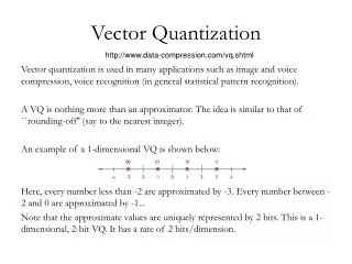
Scalar Quantiztion Process: Reminder • xk, k=1,2,…,L-1 are known as decision levels, x0=-∞, xL= ∞ • yk, k=1,2,…,L are known as representation levels • yk-yk-1, k=2,…,L is known as step size • Quantizer mapping function Y=q(X) Quantizer output is yk if the input sample X belongs to the interval Ik Ik Continuous Sample X Discrete Sample Y Quantizer q(.) yk xk-2 xk-1 xk xk+1
The Product Quantizer Assume some continuoustwo-dimensional random variable X= [X1 X2] Product Quantization Two Independently Operating Optimal Scalar Quantizers Y=q(X)=[q1(X1) q2(X2)] Since X is a two-dimensional random variable, Y is also a two-dimensional random variable. Y is a discrete two-dimensional random variable Quantization ≡ Distortion Define error (Quantizer noise) ||X-q(X)||
Product Quantiztion Process • xik, i=1,2 & k=1,2,…,Li-1 are known as decision levels for dimension i • yik, k=1,2,…,Li are known as representation levels for dimension i • Li , i=1,2 is the number of levels dedicated for dimension i y24 x23 X1 Y1 y23 Quantizer q1(X1) x22 X=[X1 X2] Y=[Y1 Y2] y22 x21 Quantizer q2(X2) y21 X2 Y2 y11 y12 y13 y14 x11 x12 x13
mX1=0, mX2=0, σ12=1, σ22=1 X2 X1 Problems with Product Quantization Quantization is based exclusively on the one-dimensional marginals. Dependencies/Correlations reflected in the joint PDF are not taken into account Why put representation points in locations that have minimal energy?
Problems with Product Quantization Even in the simplest case that the co-ordinates X1 and X2 are statistically independent, product quantization is sub-optimal. Example Suppose we need to design a 3-bit product quantizer with X1 and X2 independently and uniformly distributed between 0 and 1 Product Quantizer Optimal Quantizer X2 X2 X1 X1
Design of an Optimal Vector Quantizer • For a Decision AREAAk the representation point rk within Ak satisfies: • rk=E[X|XЄAk] • The boundary line for representation areas must be in the middle between the representation points of these areas Ak r1 r2 r3 rk=E[X|XЄAk]
Transform Coding X: Two-dimensional continuous random variable with correlated components U: U=[u1 u2]T and u1 , u2 are the eigen vectors for the covariance matrix RX Y Y=XUT is a two-dimensional continuous random variable in the transformed domain with uncorrelated components Y* Y* is a two-dimensional discrete random variable after applying the product quantization for Y. X* X*=Y*U is the transformation of Y*back to the domain of the original random variable X, X*is a two-dimensional discrete random variable UT Product Quantizer U X* Y Y*=q(Y) X
Distortion in Transform Coding d=E||X-X*||2 d=E||YU-Y*U||2 d=E||Y-Y*||2 U Since U is merely a rotation it is norm conserving d=E||Y-Y*||2 Therefore X-Distortion = Y-Distortion UT Product Quantizer U X* Y Y*=q(Y) X
Transform Coding for 2D Gaussian Assume: X1 is a one-dimensional random variable and C is a constant. Y1 is the output for an optimal scalar quatizer over X1 Claim: The scalar optimal quantizer for the random variable CX1 is CY1 Optimal Quantizer Optimal Quantizer X1 Y1 CX1 CY1
Transform Coding for 2D Gaussian Optimal Quantizer Optimal Quantizer X1 Y1 CX1 CY1 X1~ N(0,1) CX1~ N(0,C2) C=2 a c 2b 2d 2c 2a d b
Transform Coding for 2D Gaussian In transform coding of 2D Gaussian random variables, the transformed random variable with uncorrelated components is also Gaussian The quantizer in each dimension is derived from the optimal quantizer for N(0,1) UT U Y=[Y1 Y2] X* X=[X1 X2] Y* Product Quantizer