Download
1 / 12
130 likes | 515 Views
Section 5.3 ~ The Central Limit Theorem. Introduction to Probability and Statistics Ms. Young ~ room 113. Objective. Sec. 5.3. After this section you will understand the basic idea behind the Central Limit Theorem and its important role in statistics. Sec. 5.3.

E N D
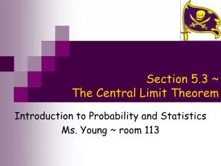
Section 5.3 ~ The Central Limit Theorem Introduction to Probability and Statistics Ms. Young ~ room 113
Objective Sec. 5.3 • After this section you will understand the basic idea behind the Central Limit Theorem and its important role in statistics.
Sec. 5.3 Visualizing the Central Limit Theorem Using Dice Suppose we roll one die 1,000 times and record the outcome of each roll, which can be the number 1, 2, 3, 4, 5, or 6.
Sec. 5.3 Visualizing the Central Limit Theorem Using Dice Now suppose we roll two dice 1,000 times and record the mean of the two numbers that appear on each roll. To find the mean for a single roll, we add the two numbers and divide by 2.
Sec. 5.3 Visualizing the Central Limit Theorem Using Dice Suppose we roll five dice 1,000 times and record the mean of the five numbers on each roll.
Sec. 5.3 Visualizing the Central Limit Theorem Using Dice Now we will further increase the number of dice to ten on each of 1,000 rolls. http://www.stat.sc.edu/~west/javahtml/CLT.html
Sec. 5.3 Visualizing the Central Limit Theorem Using Dice What do you notice about the shape of the distribution as the sample size increases? It approximates a normal distribution What do you notice about the mean of the distribution of sample means as the sample size increases in comparison to the true mean of the population (3.5)? It approaches the population mean What do you notice about the standard deviation of the distribution of means as the sample size increases? It gets smaller representing a lower variation
σ/ n Sec. 5.3 The Central Limit Theorem • The distribution of means will be approximately a normal distribution for larger sample sizes • The mean of the distribution of means approaches the population mean, μ, for large sample sizes • The standard deviation of the distribution of means approaches for large sample sizes, where σ is the standard deviation of the population and n is the sample size
Sec. 5.3 The Central Limit Theorem Side Notes • For practical purposes, the distribution of means will be nearly normal if the sample size is larger than 30 • If the original population is normally distributed, then the sample means will remain normally distributed for any sample size n, and it will become narrower • The original variable can have any distribution, it does not have to be a normal distribution
Sec. 5.3 Shapes of Distributions as Sample Size Increases
Sec. 5.3 Example 1 ~ Predicting Test Scores You are a middle school principal and your 100 eighth-graders are about to take a national standardized test. The test is designed so that the mean score is μ = 400 with a standard deviation of σ = 70. Assume the scores are normally distributed. a. What is the likelihood that one of your eighth-graders, selected at random, will score below 375 on the exam? Since the distribution is normal, we can just use z-scores to determine the percentage for one student According to the table, a z-score of -0.36 corresponds to about 36% which means that about 36% of all students can be expected to score below 375, thus there is a 36% chance that a randomly selected student will score below 375
Sec. 5.3 Example 1 ~ Predicting Test Scores • You are a middle school principal and your 100 eighth-graders are about to take a national standardized test. The test is designed so that the mean score is μ = 400 with a standard deviation of σ = 70. Assume the scores are normally distributed. • b. Your performance as a principal depends on how well your entire group of • eighth-graders scores on the exam. What is the likelihood that your group of • 100 eighth-graders will have a mean score below 375? According to the C.L.T. if we take random groups of say 100 students and study their means, then the means distribution will approach normal. Hence, the μ = 400 and its standard deviation is σ/√n = 70/√100 = 70/10 = 7 according to the C.L.T. Therefore, the z-score for a mean of 375 with a standard deviation of 7 is: The percent that corresponds to a z-score of -3.57 is less than .01%, which means that fewer than .01% of all samples of 100 students will have a mean score of 375. In other words, 1 in 5000 samples of 100 students will have a mean score of 375.