Download
1 / 16
160 likes | 183 Views
Explore strengths and weaknesses of the PPC method in analyzing ice data for IceCube, with an emphasis on ice properties and agreement with experimental data. Learn about accelerated versions, fit methods, and potential variations impacting the analysis process.

E N D
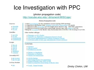
Ice Investigation with PPC (photon propagation code) http://icecube.wisc.edu/~dima/work/WISC/ppc/ Dmitry Chirkin, UW
AHA model • AHA: • method: de-convolve the smearing effect by using: • fits to the homogeneous ice (as in the ice paper) • un-smearing based on photonics • weaknesses: • code used to fit the ice is not same as used in simulation • multiple photonics issues were discovered since the model was completed unnecessarily complicated • simulation based on this model does not agree with the: • existing IceCube flasher (and standard candle?) data • muon data • neutrino data • the disagreement is not just in the bottom ice!
New fit method • Quantify the difference between simulation and data for a given flasher – receiver pair, e.g., with c2: (as in the ice paper) • sum over all receivers that have enough mean charge on nearby OMs so that the LC condition could be ignored, and charge within, say 5 and 1500 p.e. OR use soft LC data • sum over all emitters (all 60 flasher sets on string 63) • This yields 9957 pairs (terms in the c2 sum) • finally, minimize the c2 sum against the unknown ice properties: • taking as basis the 6-parameter ice model of the ice paper • by default has 171 10-meter layers with 2 unknown parameters in each
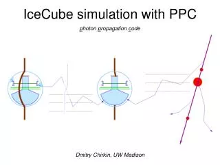
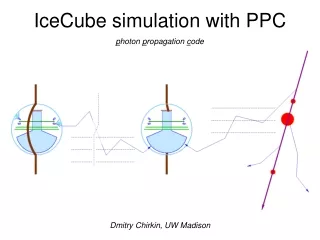
PPC • PPC: • method: • Direct fit of fully heterogeneous ice model to flasher data • strengths: • code used to fit the ice is the same as used in simulation • simple procedure, using software based on ~800 lines of c++ code • Verified extensively: • compared with photonics • compared with Tareq’s i3mcml • several different versions agree (c++, Assembly, GPU) • weaknesses: • slow (?)
Using IceCube flasher data • the waveforms obtained with hi- and low-P.E. data are of different width (due to electronics smearing effects?) • Prefer using charge information only • the total collected charge should be correct, less the saturation correction that becomes important above ~2000 p.e. (at 107 gain; by X. Bai, also see Chris Wendt and Patrick B. web pages on saturation) • most charges on the near strings are below ~500 p.e. • If that is too high, can go on to the strings farther away from flashers
Large string-to-string variations • Large string-to-string variations could be due to: • Direction of flashers relative to the observing strings • flasher-to-flasher variations in light output and width of pulse • Average behavior can be obtained with < ~20% accuracy • For the ice table fits it should also be possible to use the low-P.E. data that is planned to be collected. However, • the uncertainties on the light yield near flasher threshold are much higher, so only timing information will be used • Uncertainties in the flasher photon emission time profile are larger • cannot account for the HLC, so only SLC data is desired.
Accelerating PPC • Several accelerated versions were written: • An accelerated c++ version (factor ~1.3-1.9 faster than the standard version) • SSE-optimized versions: • A c++ version with inline assembly for the rotation code • A ppc program completely in Assembly (factor ~1.8-2.8 faster) • GPU-optimized versions: • Tareq’s i3mcml based on CUDAMCML • A version of PPC for GPU (accelerated by factor ~75-150) • compared to an npx2 node (x64 code) factor ~ 277 • with 2x configuration of GTX 295 factor ~ 554 • with 3 such cards (in a single computer) factor ~ 1662! • compared to Assembly on single I7 core factor ~ 315
Lean, mean, ice fitting machinne • Martin Merck set up a computer, “cudatest” that has: • 1 I7 CPU (4 cores, 8 threads) • 1 GTX 295 GPU by NVidia • For the iterative fitter performing the steepest descent minimization algorithm: • around 230,000,000,000 photons are simulated: 1 function evaluation 2*171 derivative calculations 40 steps along the fastest descent direction 1 final function calculation at the new minimum So, 384 function evaluations, for each 60 flashers are simulated with 107 photons each 384*60*107 = 2.3 1011. (with the 250 scaling factor this corresponds to a number of real photons of 57,600,000,000,000) per minimizer step One step completes in 4-6 hours. It takes ~10 steps for the minimizer to converge.
New ice parameters aha aha new new
Conclusions • After only 5 iterations with PPC: much better agreement at all depths • Differences up to factor ~10 in the AHA size (e.g., DOM ) are reduced to below ~20%. • ice model based on fits to in-situ light sources can describe the muon data! • fits to the flasher data with PPC are performed in one step, using same code that is used to verify other types of data (muons) • A fast version of PPC accelerates the calculation by ~1000x, making it possible to perform a fully-automated multi-ice-layer fit. • entire project is only ~1200 lines of code, easy to set up and run
Calculation speed considerations • For each iteration step: • 109 photons generated for each DOM position (factor x 60) • takes ~4 hours on 40 nodes of npx2 (with the Assembly code) • results can be obtained after only 8 iterations (and a semi-empirical correction after each step) • What we want is a fully automatic procedure that varies scattering and absorption at 60 positions (120 parameters) • a speedup of 103 - 104 is desirable. • this might be possible with running on a GPU • Tareq demonstrated 100x improvement compared to a single CPU node • PPC was also re-written to run on the GPU • also reduce the number of generated photons (factor ~10) • also further increase the DOM size (another factor ~10)