Download
1 / 52
580 likes | 1.27k Views
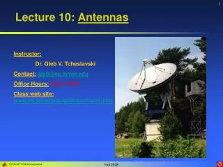
Lecture 10: Antennas. Instructor: Dr. Gleb V. Tcheslavski Contact: gleb@ee.lamar.edu Office Hours: Room 2030 Class web site: www.ee.lamar.edu/gleb/em/Index.htm. Radiation fundamentals.

E N D
Lecture 10: Antennas Instructor: Dr. Gleb V. Tcheslavski Contact:gleb@ee.lamar.edu Office Hours:Room 2030 Class web site:www.ee.lamar.edu/gleb/em/Index.htm
Radiation fundamentals Recall, that using the Poynting’s theorem, the total power radiated from a source can be found as: (10.2.1) Which suggests that both electric and magnetic energy will be radiated from the region. A stationary charge will NOT radiate EM waves, since a zero current flow will cause no magnetic field. In a case of uniformly moving charge, the static electric field: (10.2.2) The magnetic field is: (10.2.3)
Radiation fundamentals In this situation, the Poynting vector does not point in the radial direction and represent a flow rate of electrostatic energy – does not contribute to radiation! A charge that is accelerated radiates EM waves. The radiated field is: (10.3.1) Where is the angle between the point of observation and the velocity of the accelerated charge and [a] is the acceleration at the earliest time (retarded acceleration). Assuming that the charge is moving in vacuum, the magnetic field can be found using the wave impedance of the vacuum: (10.3.2) And the Poynting vector directed radially outward is: (10.3.3)
Radiation fundamentals Only accelerated (or decelerated) charges radiate EM waves. A current with a time-harmonic variation (AC current) satisfies this requirement. Example 10.1: Assume that an antenna could be described as an ensemble of N oscillating electrons with a frequency in a plane that is orthogonal to the distance R. Find an expression for the electric field E that would be detected at that location. The maximum electric field is when = 900: (10.4.1) Where we introduce the electric current density J = NQv of the oscillating current. Assuming that the direction of oscillation in the orthogonal plane is x, then (10.4.2) (10.4.3)
Radiation fundamentals The current density will become: (10.5.1) Finally, the transverse electric field is (10.5.2) The electric field is proportional to the square of frequency implying that radiation of EM waves is a high-frequency phenomenon.
Infinitesimal electric dipole antenna We assume the excitation as a time-harmonic signal at the frequency , which results in a time-harmonic radiation. The length of the antenna L is assumed to be much less than the wavelength: L << . Typically: L < /50. The antenna is also assumed as very thin: ra << . The current along the antenna is assumed as uniform: (10.6.1) For a time-harmonic excitation: (10.6.2)
Infinitesimal electric dipole antenna The vector potential can be computed as: (10.7.1) With the solution that can be found in the form: (10.7.2) Assuming a time-harmonic current density: (10.7.3) The distance from the center of the dipole R = r and k is the wave number. The volume of the dipole antenna can be approximated as dv’ = Lds’.
Infinitesimal electric dipole antenna Considering the mentioned assumptions and simplifications, the vector potential becomes: (10.8.1) This infinitesimal antenna with the current element IL is also known as a Herzian dipole. Assuming that the distance from the antenna to the observer is much greater than the wavelength (far filed, radiation field, or Fraunhofer field of antenna), i.e. r >> , let us find the components of the field generated by the antenna. Using the spherical coordinates: (10.8.2)
Infinitesimal electric dipole antenna The components of the vector potential are: (10.9.1) (10.9.2) (10.9.3) The magnetic field intensity can be computed from the vector potential using the definition of the curl in the SCS: (10.9.4)
Infinitesimal electric dipole antenna Which can be rewritten as (10.10.1) (10.10.2) (10.10.3) Note: the equations above are approximates derived for the far field assumptions. The electric field can be computed from Maxwell’s equations: (10.10.4)
Infinitesimal electric dipole antenna The components of the electric field in the far field region are: (10.11.1) (10.11.2) (10.11.3) where (10.11.4) is the wave impedance of vacuum.
Infinitesimal electric dipole antenna The angular distribution of the radiated fields is called the radiation pattern of the antenna. Both, electric and magnetic fields depend on the angle and have a maximum when = 900 (the direction perpendicular to the dipole axis) and a minimum when = 00. The blue contours depicted are called lobes. They represent the antenna’s radiation pattern. The lobe in the direction of the maximum is called the main lobe, while any others are called side lobes. A null is a minimum value that occurs between two lobes. For the radiation pattern shown, the main lobes are at 900 and 2700 and nulls at 00 and 1800. Lobes are due to the constructive and destructive interference.
Infinitesimal electric dipole antenna One of the goals of antenna design is to place lobes at the desired angles. Every null introduces a 1800 phase shift. In the far field region (traditionally, the region of greatest interest) both field components are transverse to the direction of propagation. The radiated power: (10.13.1) We have replaced the constant current by the averaged current accounting for the fact that it may have slow variations in space.
Infinitesimal electric dipole antenna Example 10.2: A small antenna that is 1 cm in length and 1 mm in diameter is designed to transmit a signal at 1 GHz inside the human body in a medical experiment. Assuming the dielectric constant of the body is approximately 80 (a value for distilled water) and that the conductivity can be neglected, find the maximum electric field at the surface of the body that is approximately 20 cm away from the antenna. The maximum current that can be applied to the antenna is 10 A. Also, find the distance from the antenna where the signal will be attenuated by 3 dB. The wavelength within the body is: The characteristic impedance of the body is:
Infinitesimal electric dipole antenna Since the dimensions of the antenna are significantly less than the wavelength, we can apply the far field approximation for = 900, therefore: An attenuation of 3 dB means that the power will be reduced by a factor of 2. The power is related to the square of the electric field. Therefore, an attenuation of 3 dB would mean that the electric field will be reduced by a square root of 2. The distance will be
Finite electric dipole antenna Finite electric dipole consists of two thin metallic rods of the total length L, which may be of the order of the free space wavelength. Assume that a sinusoidal signal generator working at the frequency is connected to the antenna. Thus, a current I(z) is induced in the rods. We assume that the current is zero at the antenna’s ends (z = L/2) and that the current is symmetrical about the center (z = 0). The actual current distribution depends on antenna’s length, shape, material, surrounding,…
Finite electric dipole antenna A reasonable approximation for the current distribution is (10.17.1) Far field properties, such as the radiated power, power density, and radiation pattern, are not very sensitive to the choice of the current distribution. However, the near field properties are very sensitive to this choice. Deriving the expressions for the radiation pattern of this antenna, we represent the finite dipole antenna as a linear combination of infinitesimal electric dipoles. Therefore, for a differential current element I(z)dz, the differential electric field in a far zone is (10.17.2)
Finite electric dipole antenna The distance can be expressed as: (10.18.1) This approximation is valid since r >> z Replacing r’ by r in the amplitude term will have a very minor effect on the result. However, the phase term would be changed dramatically by such substitution! Therefore, we may use the approximation r’ r in the amplitude term but not in the phase term. The EM field radiated from the antenna can be calculated by selecting the appropriate current distribution in the antenna and integrating (11.17.2) over z. (10.18.2)
Finite electric dipole antenna Since (10.19.1) and the limits of integration are symmetric about the origin, only a “non-odd” term will yield non-zero result: (10.19.2) The integration results in: (10.19.3) Where F() is the radiation pattern: (10.19.4)
Finite electric dipole antenna The first term, F1() is the radiation characteristics of one of the elements used to make up the complete antenna – the element factor. The second term, Fa() is the array (or space) factor – the result of adding all the radiation contributions of the various elements that form the antenna array as well as their interactions. The E-plane radiation patterns for dipoles of different lengths. infinitesimal dipole L = /2 L = L = 3/2L = 2 If the dipole length exceeds wavelength, the location of the maximum shifts.
Loop antenna A loop antenna consists of a small conductive loop with a current circulating through it. We have previously discussed that a loop carrying a current can generate a magnetic dipole moment. Thus, we may consider this antenna as equivalent to a magnetic dipole antenna. If the loops circumference C < /10 The antenna is called electrically small. If C is in order of or larger, the antenna is electrically large. Commonly, these antennas are used in a frequency band from about 3 MHz to about 3 GHz. Another application of loop antennas is in magnetic field probes.
Loop antenna Assuming that the antenna carries a harmonic current: (10.22.1) and that (10.22.2) The retarded vector potential can be found as: (10.22.3) If we rewrite the exponent as: (10.22.4) where we assumed that the loop is small: i.e. a << r, we arrive at (10.22.5)
Loop antenna Evaluating the integrals, we arrive at the following expression: (10.23.1) Recalling the magnetic dipole moment: (10.23.2) Therefore, the electric and magnetic fields are found as (10.23.3) (10.23.4) We observe that the fields are similar to the fields of short electric dipole. Therefore, the radiation patterns will be the same.
Antenna parameters In addition to the radiation pattern, other parameters can be used to characterize antennas. Antenna connected to a transmission line can be considered as its load, leading to: 1. Radiation resistance. We consider the antenna to be a load impedance ZL of a transmission line of length L with the characteristic impedance Zc. To compute the load impedance, we use the Poynting vector… If we construct a large imaginary sphere of radius r (corresponding to the far region) surrounding the radiating antenna, the power that radiates from the antenna will pass trough the sphere. The sphere’s radius can be approximated as r L2/2.
Antenna parameters The total radiated power is computed by integrating the time-average Poynting vector over the closed spherical surface: (10.25.1) Notice that the factor ½ appears since we are considering power averaged over time. This power can be viewed as a “lost power” from the source’s concern. Therefore, the antenna is “similar” to a resistor connected to the source: (10.25.2) where I0 is the maximum amplitude of the current at the input of the antenna.
Antenna parameters: Example Example 10.3: Find the radiation resistance of an infinitesimal dipole. The radiated power from the Hertzian dipole is computed as: (10.26.1) Using the free space impedance and assuming a uniform current distribution: (10.26.2) Assuming a triangular current distribution, the radiation resistance will be: (10.26.3) Small values of radiation resistance suggest that this antenna is not very efficient.
Antenna parameters For the small loop antennas, the antennas radiation resistance, assuming a uniform current distribution, will be: (10.27.1) For the large loop antennas (ka >> 1), no simple general expression exists for antennas radiation resistance. Example 10.4: Find the current required to radiate 10 W from a loop, whose circumference is /5. We can use the small loop approximation since ka = 2a/ = 0.2. The resistance: The radiated power is:
Antenna parameters 2. Directivity. The equation (10.25.1) for a radiated power can also be written as an integral over a solid angle. Therefore, we define the radiation intensity as (10.28.1) The power radiated is then: Time-averaged radial component of a Poynting vector (10.28.2) Introducing the power radiation pattern as (10.28.3) The beam solid angle of the antenna is (10.28.4)
Antenna parameters It follows from the definition that for an isotropic (directionless – radiating the equal amount of power in any direction) antenna, In(,) = 1 and the beam solid angle is A = 4. We introduce the directivity of the antenna: (10.29.1) Note: since the denominator in (10.29.1) is always less than 4, the directivity D > 1.
Antenna parameters: Example Example 10.5: Find the directivity of an infinitesimal (Hertzian) dipole. Assuming that the normalized radiation pattern is the directivity will be Note: this value for the directivity is approximate. We conclude that for the short dipole, the directivity is D = 1.5 = 10lg(1.5) = 1.76 dB.
Antenna parameters 3. Antenna gain. The antenna gain is related to directivity and is defined as (10.31.1) Here is the antenna efficiency. For the lossless antennas, = 1, and gain equals directivity. However, real antennas always have losses, among which the main types of loss are losses due to energy dissipated in the dielectrics and conductors, and reflection losses due to impedance mismatch between transmission lines and antennas.
Antenna parameters 4. Beamwidth. Beamwidth is associated with the lobes in the antenna pattern. It is defined as the angular separation between two identical points on the opposite sides of the main lobe. The most common type of beamwidth is the half-power (3 dB) beamwidth (HPBW). To find HPBW, in the equation, defining the radiation pattern, we set power equal to 0.5 and solve it for angles. Another frequently used measure of beamwidth is the first-null beamwidth (FNBW), which is the angular separation between the first nulls on either sides of the main lobe. Beamwidth defines the resolution capability of the antenna: i.e., the ability of the system to separate two adjacent targets. For antennas with rotationally symmetric lobes, the directivity can be approximated: (10.32.1)
Antenna parameters: Example Example 10.6: Find the HPBW of an infinitesimal (Hertzian) dipole. Assuming that the normalized radiation pattern is and its maximum is 1 at = /2. The value In = 0.5 is found at the angles = /4 and = 3/4. Therefore, the HPBW is HP = /2.
Antenna parameters Antennas exhibit a property of reciprocity: the properties of an antenna are the same whether it is used as a transmitting antenna or receiving antenna. 5. Effective aperture. For the receiving antennas, the effective aperture can be loosely defined as a ratio of the power absorbed by the antenna to the power incident on it. More accurate definition: “in a given direction, the ratio of the power at the antenna terminals to the power flux density of a plane wave incident on the antenna from that direction. Provided the polarization of the incident wave is identical to the polarization of the antenna.” The incident power density can be found as: (10.34.1)
Antenna parameters Assuming that the antenna is matched with the transmission line, the power received by the antenna is (10.35.1) where Ae is the effective aperture of the antenna. Maximum power can be delivered to a load impedance, if it has a value that is complex conjugate of the antenna impedance: ZL = ZA*. Replacing the antenna with an equivalent generator with the same voltage V and impedance ZA, the current at the antenna terminals will be: (10.35.2) Since ZA + ZA* = 2RA, the maximum power dissipated in the load is (10.35.3)
Antenna parameters For the Hertzian dipole, the maximum voltage was found as EL and the antenna resistance was calculated as 202(L/)2. Therefore, for the Hertzian dipole: (10.36.1) Therefore, for the Hertzian dipole: (10.36.2) In general, the effective area of the antenna is: (10.36.3) (10.36.4)
Antenna parameters 6. Friis transmission equation. Assuming that both antennas are in the far field region and that antenna A transmit to antenna B. The gain of the antenna A in the direction of B is Gt, therefore the average power density at the receiving antenna B is (10.37.1) The power received by the antenna B is: (10.37.2) The Friis transmission equation (ignoring polarization and impedance mismatch) is: (10.37.3)
Antenna arrays It is not always possible to design a single antenna with the radiation pattern needed. However, a proper combination of various types of antennas might yield the required pattern. An antenna array is a cluster of antennas arranged in a specific physical configuration (line, grid, etc.). Each individual antenna is called an element of the array. We initially assume that all array elements (individual antennas) are identical. However, the excitation (both amplitude and phase) applied to each individual element may differ. The far field radiation from the array in a linear medium can be computed by the superposition of the EM fields generated by the array elements. We start our discussion from considering a linear array (elements are located in a straight line) consisting of two elements excited by the signals with the same amplitude but with phases shifted by .
Antenna arrays The individual elements are characterized by their element patterns F1(,). At an arbitrary point P, taking into account the phase difference due to physical separation and difference in excitation, the total far zone electric field is: (10.39.1) Field due to antenna 1 Field due to antenna 2 Here: (10.39.2) The phase center is assumed at the array center. Since the elements are identical (10.39.3) Relocating the phase center point only changes the phase of the result but not its amplitude.
Antenna arrays The radiation pattern can be written as a product of the radiation pattern of an individual element and the radiation pattern of the array (array pattern): (10.40.1) where the array factor is: (10.40.2) Here is the phase difference between two antennas. We notice that the array factor depends on the array geometry and amplitude and phase of the excitation of individual antennas.
Antenna arrays: Example Example 10.7: Find and plot the array factor for 3 two-element antenna arrays, that differ only by the separation difference between the elements, which are isotropic radiators. Antennas are separated by 5, 10, and 20 cm and each antenna is excited in phase. The signal’s frequency is 1.5 GHz. The separation between elements is normalized by the wavelength via The free space wavelength: Normalized separations are /4, /2, and . Since phase difference is zero ( = 0) and the element patterns are uniform (isotropic radiators), the total radiation pattern F() = Fa().
Antenna arrays Another method of modifying the radiation pattern of the array is to change electronically the phase parameter of the excitation. In this situation, it is possible to change direction of the main lobe in a wide range: the antenna is scanning through certain region of space. Such structure is called a phased-array antenna. We consider next an antenna array with more identical elements. There is a linearly progressive phase shift in the excitation signal that feeds N elements. The total field is: (10.42.1) Utilizing the following relation: (10.42.2)
Antenna arrays the total radiated electric field is (10.43.1) Considering the magnitude of the electric field only and using (10.43.2) we arrive at (10.43.3) where (10.43.4) is the progressive phase difference between the elements. When = 0: (10.43.5)
Antenna arrays The normalized array factor: (10.44.1) The angles where the first null occur in the numerator of (10.43.1) define the beamwidth of the main lobe. This happens when (10.44.2) Similarly, zeros in the denominator will yield maxima in the pattern.
Antenna arrays Field patterns of a four-element (N = 4) phased-array with the physical separation of the isotropic elements d = /2 and various phase shift. The antenna radiation pattern can be changed considerably by changing the phase of the excitation.
Antenna arrays Another method to analyze behavior of a phase-array is by considering a non-uniform excitation of its elements. Let us consider a three-element array shown. The elements are excited in phase ( = 0) but the excitation amplitude for the center element is twice the amplitude of the other elements. This system is called a binomial array. Because of this type of excitation, we can assume that this three-element array is equivalent to 2 two-element arrays (both with uniform excitation of their elements) displaced by /2 from each other. Each two-element array will have a radiation pattern: (10.46.1)
Antenna arrays Next, we consider the initial three-element binomial array as an equivalent two-element array consisting of elements displaced by /2 with radiation patterns (10.46.1). The array factor for the new equivalent array is also represented by (10.46.1). Therefore, the magnitude of the radiated field in the far-zone for the considered structure is: (10.47.1) No sidelobes!! Element pattern F1() Array factor FA() Antenna pattern F()
Antenna arrays (Example) Example 10.8: Using the concept of multiplication of patterns (the one we just used), find the radiation pattern of the array of four elements shown below. This array can be replaced with an array of two elements containing three sub-elements (with excitation 1:2:1). The initial array will have an excitation 1:3:3:1 and will have a radiation pattern, according to (10.40.1), as: Array factor Antenna array pattern Element pattern
Antenna arrays Continuing the process of adding elements, it is possible to synthesize a radiation pattern with arbitrary high directivity and no sidelobes if the excitation amplitudes of array elements correspond to the coefficients of binomial series. This implies that the amplitude of the kth source in the N-element binomial array is calculated as (10.49.1) It can be seen that this array will be symmetrically excited: (10.49.2) Therefore, the resulting radiation pattern of the binomial array of N elements separated by a half wavelength is (10.49.3)
Antenna arrays During the analysis considered so far, the effect of mutual coupling between the elements of the antenna array was ignored. In the reality, however, fields generated by one antenna element will affect currents and, therefore, radiation of other elements. Let us consider an array of two dipoles with lengths L1 and L2. The first dipole is driven by a voltage V1 while the second dipole is passive. We assume that the currents in both terminals are I1 and I2 and the following circuit relations hold: (10.50.1) where Z11 and Z22 are the self-impedances of antennas (1) and (2) and Z12 = Z21 are the mutual impedances between the elements. If we further assume that the dipoles are equal, the self-impedances will be equal too.