Download
1 / 52
540 likes | 613 Views
Develop a simulation model to evaluate GF Auto Corporation's NPV for a new compact car over a 10-year time horizon, considering factors like fixed costs, variable production costs, selling prices, and demand fluctuations. Use financial modeling techniques to make strategic decisions.

E N D
Example 12.6 A Financial Planning Model
Background Information • General Ford (GF) Auto Corporation is trying to determine what type of compact car to develop. • Each model is assumed to generate sales for 10 years. • GF has gathered information about the following quantities through focus groups with the marketing and engineering departments.
Background Information -- continued • Fixed cost of developing car. This cost is assumed to be normally distributed with a $2.3 billion mean and a standard deviation of $0.5 billion. • Variable production cost. This cost, which includes all variable production costs required to build a single car, is normally distributed for each model during year 1 with a mean and standard deviation of $7800 and $600. Each year after year 1 the variable production cost is the previous year’s multiplied by an inflation factor. Each year this inflation factor is assumed to be normally distributed with mean 1.05 and standard deviation 0.015. All production costs are assumed to occur at the ends of the respective years.
Background Information -- continued • Selling price. The price in year 1 is already set at $11,800. After year 1 the price will increase by the same inflation factor that drives production costs. Like production costs, revenues from sales are assumed to occur at the ends of the respective years. • Demand. The demand for cars in year 1 is assumed to be normally distributed with a mean of 100,000. The standard deviation is 10,000. After year 1 the demand in the given year is assumed to be normally distributed with mean equal to the actual demand in the previous year and standard deviation 10,000. An implication of this assumption is that demands in successive years are not probabilistically independent.
Background Information -- continued • Production. In any particular year GF plans to base its production policy on the probability distribution of demand for that year - before the actual demand for that year is observed. If demand in any given year is greater than production, then the excess demand is lost. If production in any year is greater than demand, GF will sell the excess cars at an end-of-year discount of 30%. • Interest rate. GF plans to use a 10% interest rate to discount future cash flows. • Given these assumptions, GF wants to develop a simulation model that will evaluate its NPV (net present value) for this new car over the 10-year time horizon.
Developing the Spreadsheet Model • Inputs. Enter the various inputs in the shaded cell. • Production multiplier. The only real decision GF has to make is the multiplier k for its production level. To experiment with several values of this multiplier, enter the formula =RISKSIMTABLE({0.8, 1, 1.2}) in cell E20. Other (or more) values could be tried here. • Variable cost inflation factors. Rows 26-42 contain a single 10-year simulation. The approach is to enter appropriate formulas in column B and C for years 1 and 2, then copy the year 2 formulas to the columns for the other years, and finally calculate the values in rows 36, 39, 40 and 42. Begin by entering the variable production cost inflation factor relating year 2 to year 1 in cell C27 with the formula =RISKNORMAL(InflMean,InflStdev) and copying this to the rest of row 27.
Developing the Spreadsheet Model -- continued • Production quantities. The production quantity in year 1 is based on the expected demand and the standard deviation of demand in year 1, so we enter the formula =Dem1Mean+ProdFactor*Dem1StDev in cell B28. For other years, the expected demand is the previous year’s actual demand, and this is used to calculate the production quantity. Therefore for year 2, enter the formula =B29+ProdFactor*DemStDev in cell C28 and copy it across to the rest of the row 28. • Demands. Generate a demand in year 1 in cell B29 with the formula =RISKNORMAL(Dem1Mean,Dem1Stdev). As in the previous step the expected demand for year 2 is the actual demand for year 1. So generate demand for year 2 in cell C29 with the formula=RISKNORMAL(29,DemStdev), and then copy it to the rest of row 29 to generate demands for the other years.
Developing the Spreadsheet Model -- continued • Variable production costs. Generate the variable production cost for year 1 in cell B30 with the formula =RISKNORMAL(VC1Mean,VC1Stdev). Then use the inflation factor in row 27 to generate the variable production cost for year 2 in cell C30 with the formula =B30*C27 and copy this across to the rest of row 30. • Selling prices. Enter the (nonrandom) selling price for year 1 in cell B31 with the formula =Price1. Then generate the price for year 2 in cell C31 with the formula =B31*C27 and copy this across to the rest of row 31.
Developing the Spreadsheet Model -- continued • Production costs. The production cost for any year is the production quantity multiplied by the variable production cost, so enter the formula =B28*B30 in cell B33 and copy it to the rest of row 33. • Revenues. The revenues in any year are calculated in one of two possible ways. If demand is greater than production quantity, then revenue is the sales price multiplied by the production quantity. If demand is less than the production quantity, then revenue is the sales price multiplied by the demand, plus the discounted sales price multiplied by the number of cars left over. Therefore, calculate the revenue for year 1 in cell B34 with the formula=IF(B28<B29,B31*B28,B31*(B29+(1-Discount)*(B28-B29)))and copy it to the rest of row 34.
Developing the Spreadsheet Model -- continued • Fixed cost. Generate the fixed cost of developing the car in cell B36 with the formula =RISKNORMAL(FCMean,FCStdev)*1000. • NPVs. Calculate the NPV of all production costs (in millions of dollars) in cell B39 with the formula =NPV(IntRate,Costs)Similarly, enter the formula =NPV(IntRate,Revenues) in cell B40 for revenues. • Total NPV. Finally calculate the total NPV in cell B42 with the formula =RISKOUTPUT( )+B40-B36-B39
Using @Risk • Now that the spreadsheet is setup we can use the @Risk toolbar to run the simulation. • We set the number of iterations to 1000 and the number of simulations to 3. • After running @Risk, we obtain the summary measures for the total NPV shown on the next slide. • We see that the multiplier k definitely makes a difference.
@Risk Results • Here is the summary results and simulations statistics.
@Risk Results -- continued • Based on these results, GF might want to experiment with even larger values of k. • Higher values of k mean larger production quantities. • This will result in more end-of-year discounted sales, but it is evidently better than lost sales from insufficient supply. • The corresponding histogram for k = 1.2 appears on the next slide. It’s wide spread indicates the large amount of uncertainty about the 10-year NPV for this car.
@Risk Results -- continued • GF could make a lot of money, or it could lose a lot. • We entered two representative values in the Left X and the Right X boxes. • They show that the probability of a negative NPV is slightly greater than 0.22 and the probability of NPV being less than $10 million is 0.65. • We certainly would not discourage the company from proceeding with this car, because there is a lot of potential for profit, but it should also be aware of the potential for loss.
Example 12.7 A Cash Balance Model
Background Information • The Entson Company believes that it’s monthly sales during the period from November 2000 to July 2001 are normally distributed with the means and standard deviations given in the following table. • Each month Entson incurs fixed costs of $250,000. In March taxes of $150,000 and in June taxes of $50,000 must be paid. Dividends of $50,000 must also be paid in June.
Background Information -- continued • Entson estimates that its receipts in a given month are a weighted sum of sales from the current month, the previous month, and two months ago with weights 0.2, 0.6, and 0.2. In symbols, if Rt and St represent receipts and sales in month t, then Rt = 0.2St-2 + 0.6St-1 + 0.2St • The materials and labor needed to produce a month’s sales must be purchased 1 month in advance, and the cost of these averages to 80% of the product’s sales.
Background Information -- continued • At the beginning of January, 2001, Entson has $250,000 in cash. • The company would like to ensure that each month’s ending cash balance never dips below $250,000. • This means that Entson might have to take out short-term (1-month) loans. • The company would like to use simulation to estimate the maximum loan it will need to take out to meet its desired minimum cash balance.
Background Information -- continued • It would also like to see how sensitive the results are to the sales data. • In particular, considering the data in the table as a “base case”, it would like to run a simulation in which the means are 20% below the values in the table and another simulation in which the means are 20% above those in the table.
Bookkeeping • There is a considerable amount of bookkeeping in this simulation, so it is a good idea to list the events in chronological order that occur each month. • Beginning cash balance is observed. • Interest on its beginning cash balance is received. • Receipts arrive and expenses are paid (including payback of the previous month’s loan, if any, with interest) • Short term loan is taken out, if necessary • Final cash balance is observed, which becomes next month’s beginning cash balance.
CASHBAL.XLS • The inputs for this example can be found in this file. • The simulation model appears on the next slide.
Developing the Spreadsheet Model • Follow these steps to develop the spreadsheet model: • Inputs. Enter the various inputs in the shaded cells. • Scenarios. Enter the formula =RISKSIMTABLE(BaseLevList) in cell B26 This allows us to run three simulations simultaneously. The middle value, 1, corresponds to the base case. The other two values, .8 and 1.2, correspond to the scenarios in which mean sales are 20% below and 20% above the base case. • Actual sales. Generate the sales in row 30 by entering the formula =RISKNORMAL(B6*BaseLev,B7) in cell B30 and copying across.
Developing the Spreadsheet Model -- continued • Beginning cash balance. For January 2001 enter the cash balance with the formula =InitCash in cell D33. Then for the other months enter the formula =D45 in cell E33 and copy it across row 33. • Incomes. Entson’s incomes (interest on cash balances and receipts) are calculated in row 34 and 35. To calculate these enter the formulas =IntRateCash*D33 and =SUMPRODUCT(RecFactors,B30:D30) in cells D34 and D35 and copy them across the rows 34 and 35. • Expenses. Enston’s expenses are calculated in rows 37-41. Calculate these by entering the forumlas =D9, =D10, =CostPct*E30, =D44 and =D44*(IntRateLoan) in cells D37, D38, D39 and E40, and E41 and then copy them across the rows 37-41.
Developing the Spreadsheet Model -- continued • Cash balance before loan. Calculate the cash balance before the loan by entering the formula =SUM(D33:D35)-SUM(D37:D40) in cell D43 and copying it across row 43. • Amount of loan. If the value in row 43 is below the minimum cash balance ($250,000), Entson must borrow enough to bring the cash balance up to this minimum. Otherwise no loan is necessary. Therefore, enter the formula =MAX(MinCashBal-D43,0) in cell D44 and copy it across row 44. • Final cash balance. Calculate the final cash balance by entering the formula =D43+D44 in cell D45 and copying it across row 45.
Developing the Spreadsheet Model -- continued • Maximum loan. Calculate the maximum loan from January to June in cell B47 with the formula =RISKOUTPUT( )+MAX(Loans) Then calculate the total interest paid on all loans in cell B48 with the formula =RISKOUTPUT( )+SUM(IntPayments).
Using @Risk • For the settings use 1000 iterations and 3 as the number of simulations. • The results appear numerically in the following figures.
@Risk Results • The data in the Results indicates that for the base case the maximum loan varied considerably, from a low of $463,255 to a high of $1,446,719. • The average was $945,007. • They also show that when sales are below the base case, the maximum loan tends to be larger. • The opposite is true when sales are above the base case. This makes sense. • Sales generate cash, so that when sales are low, less cash is generated and higher loans are required.
@Risk Results -- continued • We also see that Entson is spending about $20,000 on average in interest on the loans, although the actual amounts vary considerably from one iteration to another. • We can also gain insights by creating a summary chart of the series of loans. • To obtain this chart, we must first identify the Loans range as an output range.
@Risk Results -- continued • After running the simulation, we can then request a summary chart of this output range. • The summary chart for the Loans range appears on the next slide. • This chart clearly shows how the loans vary through time. The middle line is the expected loan amount. The inner bands extend to one standard deviation on each side of the mean, and the outer bands extend to the 5th and 95th percentiles. • We see that the largest loans will be required in March and April.
Example 12.11 Simulating Stock Price and Options
Background Information • Attorney Sally Evans has just begun her career. At age 25, she has 40 years until retirement, but she realizes that now is the time to start investing. • She plans to invest $1000 at the beginning of each of the next 40 years. • Each year, she plans to put fixed percentages – the same each year – of this $1000 in stocks, bonds and T-bills. However, she is not sure which percentage to use. • She does have historical annual returns from stocks, bond and T-bills from 1946-1994.
RETIREMENT.XLS • This file contains the historical data for the stocks, bond and T-bills. • This file also includes inflation factors for these years. • For example, for 1993 the annual returns for stocks, bonds, and T-bills were 9.99%, 18.24% and 2.90%, and then inflation rate was 2.75%. • Sally would like to use simulation to help decide what investment weights to use, with the objective of achieving a large investment value, in today’s dollars, at the end of 40 years.
Solution • The most difficult part of the solution is settling on a way to use the historical returns and inflation factors to generate future values of these quantities. • We will use a “scenario” approach. • We think of each historical year as a possible scenario, where the scenario specifies the returns and inflation factor for that year. • Then for any future year, we randomly choose one of these scenarios, using RISKDISCRETE function.
Solution -- continued • It seems intuitive that more recent scenarios ought to have a larger chance of being chosen. • To implement this idea, we give a weight to each scenario, starting with weight 1 for 1994. Then the weight for any year is a “damping factor” times the weight from the next year. • To change these weights to probabilities, we simply divide each weight by the sum of all the weights. The damping factor we will illustrate is 0.98.
Solution -- continued • The other difficult part of the solution is knowing which investment weights to try. • This is really an optimization problem – find three weights that add to 1 and produce the largest mean final cash. • Palisades has another software package – RiskOptimizer, that solves this type of optimization-simulation problem.
RETIREMENT.XLS • The historical data and the simulation model appear on the following slides and in this file.
Developing the Spreadsheet Model • The model can be developed as follows. • Inputs. Enter the data in the shaded regions. These include the historical returns and inflation factors, the alternative sets of investment weights we plan to test, and other inputs. • Weights. The investment weights we will use for the model are in row 17. We do this with a RISKSIMTABLE and VLOOKUP combination in the usual way. Specifically, enter the formulas =RISKSIMTABLE(A10:A12) and =VLOOKUP(Index,Ltable1,B15) in cells A17 and B17, and copy the latter to the range C17:D17.
Developing the Spreadsheet Model -- continued • Probabilities. Enter value 1 in cell F69. Then enter the formula =Damper*F69 in cell F68 and copy it up to cell F21. Sum these values with the SUM function in cell F70. Then to convert them to probabilities, enter the formula =F21/$F$70 in cell G21 and copy it down to cell G69. • Scenarios. Moving to the model shown, we want to simulate 40 scenarios in columns K-O, one for each year of Sally’s investing. To do this, enter the formulas =RISKDISCRETE(Years,Probs) and =1+VLOOKUP($K20,LTable2,L$18) in cells K20 and L20, and then copy this latter formula to the range M20:O20. Make sure you understand how the RISKDISCRETE and VLOOKUP functions combine to capture the data from a randomly selected historical year.
Developing the Spreadsheet Model -- continued • Beginning, ending cash. The bookkeeping part is straightforward. Begin by entering the formula =Invest in cell J20 for the initial investment. Then enter the formulas =J20*SUMPRODUCT(Weights,L20:N20) and =Invest+P20 in cells P20 and J21 for ending cash in the first year and beginning cash in the second year. The former shows how the beginning cash grows in a given year. The latter implies that Sally reinvests her previous money, plus she invests a new $1000. Copy these formulas down column J and P. • Deflators. We eventually want to deflate future dollars to today’s dollars. The proper way to do this is to calculate deflators. Do this by entering the formula =1/O20 in cell Q20. Then enter the formula Q20/O21 in cells Q21 and copy it down.
Developing the Spreadsheet Model -- continued • Summary measures. For any time horizon specified in cell B6, we can pick off the information we need with a third VLOOKUP. Do this by entering the formulas =VLOOKUP(Horizon,LTable3,8), =VLOOKUP(Horizon,LTable3,9), and =RISKOUTPUT( )+K13*K14 in cells K13-K15. This last quantity is the output we will examine with @Risk.
@Risk Results • We set the number of iterations to 1000 and the number of simulations to 3. • Summary results appear here. The first simulation, which invests the most heavily in stocks, is easily the winner.
@Risk Results -- continued • The histogram for simulation 1, shown on the next slide, indicates the tremendous amount of variability – and skewness – in the distribution of final cash. • A useful concept we might introduce here is value at risk (VAR). It is defined as the 5th percentile of a distribution and is often the value investors worry about.