Quantum Path Integral Techniques in Financial Option Pricing Applications
This paper presents a detailed exploration of the application of path integrals, a central concept in quantum mechanics, in the field of financial option pricing. By examining fundamental principles and methodologies, such as the Black-Scholes model and Brownian motion, we demonstrate how quantum mechanical approaches can provide insights into price fluctuations and decision-making in financial contexts. The findings contribute to our understanding of risk management in financial markets through a quantum framework, enhancing the sophistication of financial models using theoretical physics concepts.

Quantum Path Integral Techniques in Financial Option Pricing Applications
E N D
Presentation Transcript
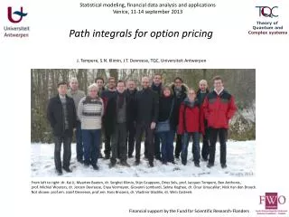
Statistical modeling, financial data analysis and applications Venice, 11-14 september 2013 Theory of Quantum and Complex systems Path integrals for option pricing J. Tempere, S.N. Klimin, J.T. Devreese, TQC, UniversiteitAntwerpen January 2013 From left to right: dr. Kai Ji, Maarten Baeten, dr. SergheiKlimin, StijnCeuppens, Dries Sels, prof. Jacques Tempere, Ben Anthonis, prof. MichielWouters, dr. JeroenDevreese, EnyaVermeyen, Giovanni Lombardi, Selma Koghee, dr. OnurUmucalilar, Nick Van den Broeck. Not shown: prof.em. JozefDevreese, prof.em. FonsBrosens, dr. Vladimir Gladilin, dr. WimCasteels Financial support by the Fund for Scientific Research-Flanders
Introduction: quantum mechanics with path integrals Two alternatives: add the amplitudes 1 B A 2
Introduction: quantum mechanics with path integrals x Many alternatives: add the amplitudes B A
Introduction: quantum mechanics with path integrals x Many alternatives: add the amplitudes B A t
Introduction: quantum mechanics with path integrals Many alternatives: add the amplitudes x is called the path integral propagator x(t) The amplitude corresponding to a givenpathx(t) is Here, S is the action functional: WithL the Lagrangian, eg. B A t H. Kleinert, Path Integrals in Quantum Mechanics, Statistics, Polymer Physics, and Financial Markets, 5th ed. (World Scientific, Singapore, 2009)
Options: the right to buy/sell in the future at a fixed price Main question in option pricing: how much is this ‘right to buy in the future’ worth? sT=730 p K=630 1-p s0=610 sT=530 Expected payoff: p100+(1p)0 One year from now, you will require 100 tonne of steel; how do you deal withpossiblepricefluctuations? 1. Decide a price now, say 630 EUR/tonne. Rather than a contract to get steel in one year at 630 EUR/tonne, it is better to obtain the right, not the obligation to buy steel at 630 EUR/tonneone year from now. This is called an ‘option contract’. All types exist, eg.also the right to sell, with different times, and for different underlying assets.
The ‘standard model’ of option pricing: Black-Scholes We work with the logreturn and model the changes in the value of the underlying asset as a Brownian random walk time x From the payoff at the final position, work a step back to obtain a differential equation p p 1-p 1-p Binomial tree method: see eg. Options, Futures, and Other Derivatives by John C. Hull (Prentice Hall publ.)
The ‘path-centered’ point of view on Black-Scholes Rather than 2 possible futures, there are many – but they can bee seen as a limit of many small ‘binomial’ steps according to the central limit theorem, the outcome is Gaussian fluctuations The probability to end up in xT is also given by the sum over all paths that end up there, weighed by the probability of these paths We work with the logreturn and model the changes in the value of the underlying asset as a Brownian random walk x time x Take the sum over all paths: this is the price propagator from t=0 to t=T. (note: in this example there would already be 212 possible paths…) p 1-p etc.
The ‘path-centered’ point of view on Black-Scholes Rather than 2 possible futures, there are many – but they can bee seen as a limit of many small ‘binomial’ steps according to the central limit theorem, the outcome is Gaussian fluctuations The probability to end up in xT is also given by the sum over all paths that end up there, weighed by the probability of these paths We work with the logreturn and model the changes in the value of the underlying asset as a Brownian random walk x time x Quantum Many alternatives: add the amplitudes this Feynman path integral determines the propagator x(t) x0 xT The amplitude for a given path is a phase factor : where S is the action functional , fixed by integrating the Lagrangian along the path, eg. for a free particle:
The ‘path-centered’ point of view on Black-Scholes Rather than 2 possible futures, there are many – but they can bee seen as a limit of many small ‘binomial’ steps according to the central limit theorem, the outcome is Gaussian fluctuations The probability to end up in xT is also given by the sum over all paths that end up there, weighed by the probability of these paths We work with the logreturn and model the changes in the value of the underlying asset as a Brownian random walk x time x Stochastic Many alternatives: add the probabilities this Wienerpath integral determines the propagator x(t) x0 xT The amplitude for a given path is a phase factor : where S is the action functional , fixed by integrating the Lagrangian along the path, eg. for a free particle:
The ‘path-centered’ point of view on Black-Scholes Rather than 2 possible futures, there are many – but they can bee seen as a limit of many small ‘binomial’ steps according to the central limit theorem, the outcome is Gaussian fluctuations The probability to end up in xT is also given by the sum over all paths that end up there, weighed by the probability of these paths We work with the logreturn and model the changes in the value of the underlying asset as a Brownian random walk x time x Stochastic Many alternatives: add the probabilities this Wienerpath integral determines the propagator x(t) x0 xT The probabilityfor a given path is a real number: where S is the action functional , fixed by integrating the Lagrangian along the path, eg. for a free particle:
The ‘path-centered’ point of view on Black-Scholes Rather than 2 possible futures, there are many – but they can bee seen as a limit of many small ‘binomial’ steps according to the central limit theorem, the outcome is Gaussian fluctuations The probability to end up in xT is also given by the sum over all paths that end up there, weighed by the probability of these paths We work with the logreturn and model the changes in the value of the underlying asset as a Brownian random walk x time x Stochastic Many alternatives: add the probabilities this Wienerpath integral determines the propagator x(t) x0 xT The probabilityfor a given path is a real number: where S is the action functional , fixed by integrating the Lagrangian along the path, eg. for the BS model:
The ‘path-centered’ point of view on Black-Scholes Rather than 2 possible futures, there are many – but they can bee seen as a limit of many small ‘binomial’ steps according to the central limit theorem, the outcome is Gaussian fluctuations The probability to end up in xT is also given by the sum over all paths that end up there, weighed by the probability of these paths We work with the logreturn and model the changes in the value of the underlying asset as a Brownian random walk x Black-Scholes: The Galton board Many alternatives: add the probabilities this Wienerpath integral determines the propagator The probabilityfor a given path is a real number: where S is the action functional , fixed by integrating the Lagrangian along the path, eg. for the BS model: The application of path integrals to option prices in BS has been pioneered by various authors: Dash, Linetsky, Rosa-Clot, Kleinert.
The ‘path-centered’ point of view on Black-Scholes Rather than 2 possible futures, there are many – but they can bee seen as a limit of many small ‘binomial’ steps according to the central limit theorem, the outcome is Gaussian fluctuations The probability to end up in xT is also given by the sum over all paths that end up there, weighed by the probability of these paths We work with the logreturn and model the changes in the value of the underlying asset as a Brownian random walk x Fisher Black & Myron Scholes, "The Pricing of Options and Corporate Liabilities". Journal of Political Economy 81 (3): 637–654 (1973). Robert C. Merton, "Theory of Rational Option Pricing“, Bell Journal of Economics and Management Science (The RAND Corporation) 4 (1): 141–183 (1973).
Part III: Some advantages of the path integral point of view
Two problems with the standard model Free particle propagator Black-Scholes option price Problem 1: The fluctuations are not Gaussian Black-Scholes-Merton model Δx Δx Problem 2: Not all options have a payoff that depends only on x(t=T), many options have a path-dependent payoff, i.e. payoff is a functional of x(t).
Two problems with the standard model Free particle propagator Black-Scholes option price Problem 1: The fluctuations are not Gaussian Problem 2: Not all options have a payoff that depends only on x(t=T), many options have a path-dependent payoff, i.e. payoff is a functional of x(t). x Asian option: payoff is a function of the average of the underlying price? xA xB t
Improving Black-Scholes : stochastic volatility Heston model Black-Scholes-Merton model Δx Δx Δx t vt t xt with z = (v/)1/2 The Heston model treats the variance as a second stochastic variable, satisfying its own stochastic differential equation: t t two particle problem the ‘volatility of the volatility’ mean reversion rate mean reversion level
Improving Black-Scholes : stochastic volatility Δx vt xt with z = (v/)1/2 From the infinitesimal propagator of the stochastic process we identify the following Lagrangian that corresponds to the same propagator: t t two particle problem
Improving Black-Scholes : stochastic volatility Heston model Black-Scholes-Merton model Δx Δx Δx t vt t xt with z = (v/)1/2 t t two particle problem : free particle strangely coupled to a radial harmonic oscillator
Improving Black-Scholes : stochastic volatility Heston model Black-Scholes-Merton model Δx Δx Δx t vt t xt with z = (v/)1/2 t t two particle problem : free particle strangely coupled to a radial harmonic oscillator
Improving Black-Scholes : stochastic volatility Heston model Black-Scholes-Merton model Δx Δx Δx t vt t xt with z = (v/)1/2 t t two particle problem : free particle strangely coupled to a radial harmonic oscillator Details: D.Lemmens, M. Wouters, JT, S. Foulon, Phys. Rev. E 78, 016101 (2008).
BS Add stoch vol. Add jump diff. Kou Heston Other improvements to Black-Scholes A) Stochastic Volatility * Heston model: * Hull-White model * Exponential Vasicek model B) Jump Diffusion (and Levy models) again a zoo of proposals poisson process H. Kleinert, Option Pricing from Path Integral for Non-Gaussian Fluctuations.Natural Martingale and Application to Truncated Lévy Distributions , PhysicaA 312, 217 (2002).
Other models and other tricks Improvements to Black-Scholes ...translate into ...to which quantum mechanics physical actionssolving techniques can be applied A) Stochastic Volatility 1. Heston model free particle coupled to exact solution radial harmonic oscillator B) Stochastic volatiltiy + Jump Diffusion 2. Exponential Vasicek model particle in an exponential perturbational gauge field generated by (Nozieres – Schmitt-Rink free particle expansion) 3. Kou and Merton’s models particle in complicated variational (Jensen-Feynman potential (not previously variational principle) studied) References 1. D. Lemmens, M. Wouters, J. Tempere, S. Foulon, Phys. Rev. E 78 (2008) 016101. 2. L. Z. Liang, D. Lemmens, J. Tempere, European Physical Journal B 75 (2010) 335–342. 3. D. Lemmens, L. Z. J. Liang, J. Tempere, A. D. Schepper, Physica A 389 (2010) 5193 – 5207.
More complicated payoffs ‘Plainvanilla’ or simple options have a payoffthatonlydepends on the value of the underlying at expiration, x(t=T). For such options we have: • Many other option contracts have a payoff that depends on the entire path, such as: • Asian options: payoff depends on the average price during the option lifetime • Timer options: contract duration depends on a volatility budget • Barrier options: contract becomes void if price goes above/below some value • For such options, the price is given by • Feynman-Kac ‘interpretation’ include payoff in the path weight:
Part IV: A concrete and recent example: Timer options Timer options have an uncertain expiry time, equal to the time at which a certain “variance budget” has been used up.
The Duru-Kleinert transformation ‘clock’ time is a functional of the path followed: x t x(t) x0 with and F>0 xT final time depends on path q q() qB qA H. Duru and H. Kleinert, Solution of the Path Integral for the H-Atom, Phys. Letters B 84, 185 (1979). H. Duru and N. Unal, Phys. Rev. D 34, 959 (1986).
The Duru-Kleinert transformation This transformation results in the equivalency between the following two path integrals: F(q) can be chosen to regularize a singular potential. This technique was used to solve the propagator of the electron in the hydrogen atom, transforming the a 3D singular potential into a 4D harmonic oscillator problem. H. Duru and H. Kleinert, Solution of the Path Integral for the H-Atom, Phys. Letters B 84, 185 (1979). H. Duru and N. Unal, Phys. Rev. D 34, 959 (1986).
More complicated payoffs: timer option Timer options have an uncertain expiry time, equal to the time at which a certain pre-specified “variance budget” has been used up. Their description requires a stochastic volatility model: The expiry time is determined by the variance budget B : This now defines a Duru-Kleinert pseudotime ! L. Z. J. Liang, D. Lemmens, and J. Tempere, Physical Review E 83, 056112 (2011).
More complicated payoffs: timer option Timer options have an uncertain expiry time, equal to the time at which a certain pre-specified “variance budget” has been used up. Their description requires a stochastic volatility model: The Duru-Kleinert transformation has a well defined inverse . Denoting and we find that these obey new SDE’s: now X and V evolve up to a fixed time, L. Z. J. Liang, D. Lemmens, and J. Tempere, Physical Review E 83, 056112 (2011).
More complicated payoffs: timer option The 3/2 model: results in a particle in a Morse potential. The Heston model results here in particle in a Kratzer potential L. Z. J. Liang, D. Lemmens, and J. Tempere, Physical Review E 83, 056112 (2011).
St t Conclusions Fluctuating paths in finance are described by stochastic models, which can be translated to Lagrangians for path integration. Path integrals can solve in a unifying framework the two problems of the ‘standard model of option pricing’: 1/ The real fluctuations are not gaussian 2/ New types of option contracts have path- dependent payoffs D. Lemmens, M. Wouters, JT, S. Foulon, Phys. Rev. E 78, 016101 (2008); J.P.A. Devreese, D. Lemmens, JT, PhysicaA 389, 780-788 (2010); L. Z. J. Liang, D. Lemmens, JT, European Physical Journal B 75, 335–342 (2010); L. Z. J. Liang, D. Lemmens, JT, Physical Review E 83, 056112 (2011). D. Lemmens, L. Z. J. Liang, JT, A. D. Schepper, Physica A 389, 5193–5207 (2010);