Download
1 / 19
190 likes | 356 Views
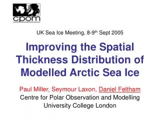
Improving the Spatial Thickness Distribution of Modelled Arctic Sea Ice. UK Sea Ice Meeting, 8-9 th Sept 2005. Paul Miller, Seymour Laxon, Daniel Feltham Centre for Polar Observation and Modelling University College London. Motivation.

E N D
Improving the Spatial Thickness Distribution of Modelled Arctic Sea Ice UK Sea Ice Meeting, 8-9th Sept 2005 Paul Miller, Seymour Laxon, Daniel Feltham Centre for Polar Observation and Modelling University College London
Motivation • Rothrock et al., (2003) showed Arctic sea ice thickness as predicted by various models • Significant differences, both in the mean and anomaly of ice thickness during the last 50 years • Causes of differences not well understood, but there is both parameter and forcing uncertainty • How can we reduce this uncertainty and increase our confidence in conjectures based on model output?
Reducing Parameter Uncertainty in Sea Ice Models • Use one of the best available sea ice models (CICE) and force it with the best available fields (ERA-40 & POLES) • Optimise and validate the model using a comprehensive range of sea ice observations: • Sea ice velocity, 1994-2001 (SSM/I + buoy + AVHRR, Fowler, 2003,NSIDC) • Sea ice extent, 1994-2001 (SSM/I, NSIDC) • Sea ice thickness, 1993-2001 (ERS radar altimeter, Laxon et al., 2003) We used this model and forcing to reduce uncertainty surrounding sea ice model parameters
Parameter Space We explored the model’s multi-dimensional parameter space to find the ‘best’ fit to the observational data • Our parameter space has three dimensions • Uncertainty surrounds correct values to use • Space includes commonly-used values • 168 model runs needed to optimise model Albedo, ice 0.62 0.54 0.0003 Ice strength, P* 0.0016 2.5 100 (kPa) Air drag coefficient, Cair
Arctic Basin Ice Thickness(<81.5oN) Miller et al 2005a {ice, Cair, P*} = {0.56, 0.0006, 5 kPa}
Validation Using ULS Data from Submarine Cruises • We consider data from 9 submarine cruises between 1987 and 1997 • Rothrock et al. (2003) used this data to test their coupled ice-ocean model • Modelled cruise means of ice draft are in good agreement with ULS observations Rothrock et al., 2003, JGR, 108(C3), 3083 R = 0.98 RMS difference = 0.28m
Spatial Draft Discrepancy Rothrock et al., 2003, JGR, 108(C3), 3083 Optimised CICE Model
Sea Ice Rheology 2 e=√.5 S 1 P/2 • CICE sea ice rheology is plastic • CICE has an elliptical yield curve, with ratio of major to minor axes, e (Hibler, 1979) • Maximum shear strength determined by P*, thickness, concentration and e • Decreasing e reduces ice thickness in the western Arctic and increases it near the Pole S e=2 C
Spatial Draft Discrepancy e=2 e=√.5
Improvements Due to Increased Shear Strength e = √.5 e = 2 Improved Cruise Averages Improved Zonal Averages
Model vs ERS Mean Winter Ice Thickness (<81.5oN) e = 2 e = √.5 Model-Satellite Thickness (m)
Truncated Yield Curve 2 1 S e=2 e=√.5
Truncated Yield Curve 2 1 S e=2 e=√.5 Truncated
Truncated Yield Curve 2 1 S e=2 e=√.5 Truncated < 80% Ice Concentration
Arctic Basin Ice Thickness Since 1980 e = 2 e = √.5 e = √.5 (Truncated for IC < 80%)
Conclusions • Initial work reduced parameter uncertainty in a stand-alone sea ice model • Observations of thickness/draft from submarine cruises were used to independently test the optimised model • By increasing the shear strength (by changing e from 2 to .5), we reproduced the observed spatial distribution of ice draft • Found that some tensile strength is necessary • These results are in press, Miller et al 2005b
Paul Miller, Seymour Laxon, Daniel Feltham Centre for Polar Observation and Modelling, UCL
Slide 5 Melt Season Length Ice Concentration Ice Motion • Extend observational validation back to mid-1980’s using intermittent submarine data • Use optimised model to examine changes in radiative, thermal, and mechanical forcing to determine primary mechanisms in ice mass change from 1948 - present
ERS-derived Mean Winter Ice Thickness e = 2 e = √.5 Model-Observed Thickness (m)