Queuing Theory for System Performance Evaluation
720 likes | 754 Views
Queuing Theory explores waiting lines, vital for predicting and assessing system performance. Learn about models, assumptions, and values. Discover how to calculate arrival rates and utilization in queuing systems.

Queuing Theory for System Performance Evaluation
E N D
Presentation Transcript
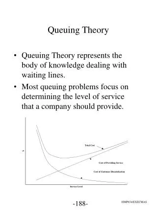
Queuing Theory • Queuing theory is the mathematics of waiting lines. • It is extremely useful in predicting and evaluating system performance. • Queuing theory has been used for operations research. Traditional queuing theory problems refer to customers visiting a store, analogous to requests arriving at a device.
Long Term Averages • Queuing theory provides long term average values. • It does not predict when the next event will occur. • Input data should be measured over an extended period of time. • We assume arrival times and service times are random.
Assumptions • Independent arrivals • Exponential distributions • Customers do not leave or change queues. • Large queues do not discourage customers. Many assumptions are not always true, but queuing theory gives good results anyway
Queuing Model Q W λ S Tw Tq
Interesting Values • Arrival rate () — the average rate at which customers arrive. • Service time (s) — the average time required to service one customer. • Number waiting (W) — the average number of customers waiting. • Number in the system (Q) — the average total number of customers in the system.
More Interesting Values • Time in the system (Tq) the average time each customer is in the system, both waiting and being serviced. • Time waiting (Tw) the average time each customer waits in the queue. Tq = Tw + s
Arrival Rate • The arrival rate, λ, is the average rate new customers arrive measured in arrivals per time period. Common units are access/second • The inter-arrival time, a, is the average time between customer arrivals. It is measured in time per customer. A common unit would be seconds/access. a = 1 / λ
Try it • Measured over a half hour period, a performance monitor shows that the hard drive received 12,600 I/O requests. • What is the arrival rate for the disk?
Random Values • We assume that most of the events we are interested in occur randomly. • Time of a request to a device • Time to service a request • Time user makes a request • Although events are random, we may know the average value of the times and their distribution. • If you flip a coin, you will get heads 50% of the time.
Exponential Distribution • Many of the random values are exponentially distributed. Frequency of Occurrence = e-t • There are many small values and a few large values. • The inter-arrival time of customers is naturally exponentially distributed.
Poisson Arrival Rate If customers are arriving at the exponentially distributed rate , then the probability that there will be k customers after time t is:
Math Notes 0! = 1! = 1 X0 = 1 X1 = X
Poisson Example • A networked printer usually gets 15 print jobs every hour. The printer has to be turned off for 10 minutes for maintenance. What is the probability that nobody will want to use the printer during that time?
Poisson Solution • A networked printer usually gets 15 print jobs every hour. The printer has to be turned off for 10 minutes for maintenance. What is the probability that nobody will want to use the printer during that time? • The arrival rate is 15/60 = 0.25 jobs/min.
Try It • On the average, 4 I/O request are sent to the disk every second. • What is the probability that no I/O requests are sent to the disk in a second? • What is the probability that one I/O request is sent to the disk in a second? • What is the probability that two or more I/O requests arrive every second?
Expected Number of Arrivals If customers are arriving at the exponentially distributed rate , how many customers should you expect to arrive in time t? Expected = * t For the printer problem with an arrival rate = 0.25, in 10 minutes we should expect 2.5 jobs to arrive
Queuing Models Queuing systems are usually described by three values separated by slashes Arrival distribution / service distribution / # of servers where: • M = Markovian or exponentially distributed • D = Deterministic or constant. • G = General or binomial distribution
Common Models • The simplest queuing model is M/M/1 where both the arrival time and service time are exponentially distributed. • The M/D/1 model has exponentially distributed arrival times but fixed service time. • The M/M/n model has multiple servers.
Why is there Queuing? • The arrivals come at random times. • Sometimes arrivals are far apart. Sometimes many customers arrive at almost the same time. When more customers arrive in a short period of time than can be serviced, queues form. • If the arrival rate was not random, queues would not be created.
Utilization • Utilization (represented by the Greek letter rho, ρ) is the fraction of time the server is busy. • Utilization is always between zero and one 0 ≤ ρ≤ 1 • If a bank teller spends 6 hours out of an 8 hour day counting money, her utilization is 6/8 = 0.75
Calculating Utilization • Utilization can be calculated from the arrival rate and the service time. It is important that the units of both the arrival rate and the service time be identical. It may be necessary to convert these values to common units.
Little’s Formula • The number in the system is equal to the arrival rate times the average time a customer spends in the system. Q = λ * Tq • This is also true for just the queue. W = λ * Tw
Application of Little’s Formula • Multiplying the formulas on the left by λ gives the formula on the right.
Solution Process • Determine what quantities you need to know. • Identify the server • Identify the queued items • Identify the queuing model • Determine the service time • Determine the arrival rate • Calculate • Calculate the desired values
Example • Consider a disk drive whose hardware can complete an average request in 10 ms. The time to complete a request is exponentially distributed. Over a period of 30 minutes, 117,000 requests were made to the disk. • How long did it take to complete the average request? • What is the average number of queued requests?
Solution • Determine what quantities you need to know. • The average request time is Tq • The number of queued jobs is W • Identify the server • The disk drive is the server • Identify the queued items • Disk requests • Identify the queuing model • M/M/1
Solution (cont.) • Determine the service time S = 10 ms = 0.01 sec / request • Determine the arrival rate λ = 117,000 request / (30 min * 60 sec/min) = 65 requests / sec • Calculate ρ = λ*s = 0.01 sec/request * 65 req/sec = 0.65
Solution (cont.) • Time to complete the average request The average length of the queue
Try It • On the average a printer receives one print request every two minutes. It takes the printer an average of 45 seconds to print the output. • How long does it take a user to get their output, from request to completion?
Number in the System • The value Q represents the average number of jobs in the system, both waiting and being served. • There are not always Q jobs in the system. Sometimes there are more, sometimes less. Q is the average.
Queue Size Probabilities The probability that there are exactly N jobs in the system is given by Summing the probabilities for individual cases gives the probability of N or less customers in the system
Large Queue Probabilities • The probability that there are more than N customers in the system is the sum of the probabilities from N-1 to ∞. • Remembering that the sum of all probabilities is one, the probability that there are more than N customers in the system is:
Example Continued • In the previous disk example, what is the probability that a request does not get queued? • A job can get serviced immediately if there are zero jobs in the system.
Accuracy and Significant Digits • Just because my calculator displays a 10 digit number does not mean the answer is accurate to 10 digits. • Your answer can only be as accurate as your input data. If your data has three significant digits, your answer cannot have more than three digits. • Always use as much accuracy as possible in these calculations and round off only at the end.
Constant Service Time • In some systems the service time is always a constant. The M/D/1 model is used for constant service time. • There is less randomness in the system. • The wait time will be less.
M/D/1 Example • An ATM network sends 53 byte packets over a 155 Mb/sec line. It always takes 2.74 μs to send a packet. Each second 145,000 packets are sent. How long does a packet wait to be sent?
M/D/1 Solution • Determine what quantities you need to know. The average time spent in the queue, Tw. • Identify the server The transmission line. • Identify the queued items Packets (not bits or bytes) • Identify the queuing model M/D/1
M/D/1 Solution • Determine the service time 2.74x10⁻⁶ seconds • Determine the arrival rate 145,000 packets/second • Calculate = 145,000 * 2.74x10-6 = 0.3973 • Calculate the desired values
Try It • On the average a printer receives one print request every two minutes. It always takes the printer exactly 45 seconds to print the output. • How long does it take a user to get their output, from request to completion?
Multiple Servers S λ S S
Multiple Servers • Customers arrive and join a single queue. • Whenever any of the servers is idle, it serves the first customer on the single queue. • All of the servers must be identical. Any customer can be served by any server. • When there are N servers, the model is M/M/N
Multiple Server Utilization • The server utilization for an N server system is: This is the average utilization for all N servers.
Intermediate Value K • To make calculations easier, we first compute the value K.
K Calculation • The first term (i = 0) is always 1 • Note that the value in the denominator is equal to the numerator plus the last term. • Since the denominator is always larger than the numerator, the value K must always be less than 1. • The value K is an intermediate that simplifies calculations. It has no intrinsic meaning.
