MPB Supply Side Implications

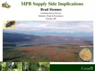
1. MPB Supply Side Implications Brad Stennes Canadian Forest Service Industry, Trade & Economics Victoria, BC

2. Outline of Talk • Brief Description of model • What we are examining – future harvest scenario, species mix and product supply implications • Results • Implications

3. Transport Model • 10 year recursive model run • Splits province into 29 current forest districts. Scaling up or down not a problem. • Fibre supply and demand characterized over time in each district. • Transport links (distance and cost) defined within districts, between districts and from district to markets.

4. Model Summary (II) Max: TR – TC St: • Resource Constraints • Capacity Constraints • Market Constraints • For this analysis harvests by species in each district are exogenously set.

5. Fibre Supply (I) • Harvests are split into 3 species groups for each forest district – pine, other coniferous, deciduous. Harvest data used for initial 2 years, then harvest assumption used for 2007-2013. • For this run future harvests based on timber supply projections by the BC MOFR, Timberline (for the Council of Forest Industries) – our final simulation year is based on their yr 16 assumed harvest.

6. Fibre Supply (II) • Harvested logs are either processed locally, transported to mills in other regions or exported directly (anything leaving BC is defined as export). • As processing occurs all co-product streams are accounted for – chips, woody residuals and bark. • Intermediate products used within model (endogenously) to produce pulp, pellets, MDF and energy (in mills or regional for sale to grid).

7. Changes over Time • The proportion of lpp increases until the last period when it falls significantly. • Recovery rates for lpp decline to a 85% of non lpp in the final period.

8. Log Quality @ 5 Years

9. Transport Functions • Transport cost functions take basic form: TC = a + bD Where: TC is total transport cost a is fixed cost b is per km costs D is one-way distance in km • We have developed independent functions for logs, lumber, chips and other residuals. • Cost of fuel in transport has been characterized => can model impact of fuel inflation on transport costs from our 2004 start year

10. Demand (I) • Demand for logs and “intermediate” products can come internally from processing demand in districts (defined by capacity – sawmills, “other roundwood”, plywood, OSB, MDF, chip mills, pellet mills, kraft pulp, mech pulp, mill energy and stand alone energy). • Also sell “final” products and generate revenue (enter the objective function) – logs, lumber, plywood, pulp, pellets, OSB, MDF and “Other” roundwood products.

11. Demand (II) • No exogenous pricing of intermediate products – values determined endogenously based on costs and final product revenues. • Lumber to US market is “price responsive” through a stepped excess demand function (used existing SPE model to develop)

12. Northern Interior Central Interior Southern Interior Coast

13. Results for Wemme Runs

14. BC Interior Harvests Over Simulation Period

15. Regional Production Changes

16. Changes in Processing Location • Share of BC production will move from Northern & Central Interior to South. • Largest dislocation in “BC Timber Basket” • Northern Interior remains the largest producer.

17. Changes in Processing Location (II) • Reductions in pulp production do not necessarily occur closer to area with large harvest reductions. • Reduction in pulp production on coast • Quesnel district, with the largest harvest reduction maintains pulp production in model – centrally located wrt to sawmill capacity.

18. Excess Capacity • When supply reductions occur there will be considerable excess processing capacity. • Average mill sizes (2005 BCMOFR) are • 200 million bf - Northern Interior • 100 million bf - Central Interior • 70 million bf – Southern Interior

19. US SWL Exports at Start, Mid and End of Time Period 2015-2020 Period

20. Results – Lumber cost implications • Processing costs rise as dead pine dominates timber supply & logs transported further afield. • Then when dead pine has worked its way out the system, costs fall as recovery increases, logs processed closer to harvest site and production occurs closer to final market (South).

21. Added Supply Issues • Increased competition for residual and chip streams from bioenergy, bioproduct sectors • large problem when production falls off • Eastern Canada Harvest Reductions. • Beetle “Clearly” Moving East – Alberta will have disruptions as well.

22. Lodgepole pine Jack pine Mountain pine beetle • Mountain pine beetle only occupies a fraction of its potential range

23. Summary • The MPB has resulted in a spike in product supply which will be followed by a significant decline. • The largest reductions in lumber production are in the Northern and Central Interior. • Exports of lumber from BC to the US will fall by a third.

24. Summary (II) • Optimistic future harvest levels? • If product prices remain low then the economic timber supply will be much lower than we have modelled here.

26. Extra Slides

27. SPE Model • Use our existing SPE trade model to develop: • A stepped excess demand function for lumber to US market in our transport model.