Analytical Solution for the Optimal Service Level
190 likes | 392 Views
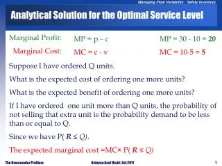
Analytical Solution for the Optimal Service Level. Marginal Profit: Marginal Cost :. MP = p – c MC = c - v. MP = 30 - 10 = 20 MC = 10-5 = 5. Suppose I have ordered Q units. What is the expected cost of ordering one more units? What is the expected benefit of ordering one more units?

Analytical Solution for the Optimal Service Level
E N D
Presentation Transcript
Analytical Solution for the Optimal Service Level Marginal Profit: Marginal Cost: MP = p – c MC = c - v MP = 30 - 10 = 20 MC = 10-5 = 5 Suppose I have ordered Q units. What is the expected cost of ordering one more units? What is the expected benefit of ordering one more units? If I have ordered one unit more than Q units, the probability of not selling that extra unit is the probability demand to be less than or equal to Q. Since we have P( R ≤ Q). The expected marginal cost =MC× P( R ≤ Q)
Analytical Solution for the Optimal Service Level If I have ordered one unit more than Q units, the probability of selling that extra unit is the probability of demand to be greater than Q. We know that P(R > Q) = 1- P(R ≤ Q). The expected marginal benefit = MB× [1-Prob.( r ≤ Q)] As long as expected marginal cost is less than expected marginal profit we buy the next unit. We stop as soon as: Expected marginal cost ≥ Expected marginal profit.
Prob(R ≤ Q*) ≥ Analytical Solution for the Optimal Service Level MC×Prob(R≤ Q*) ≥ MP×[1 – Prob( R≤ Q*)] MP = p – c = Underage Cost = Cu MC = c – v = Overage Cost = Co
Marginal Value: The General Formula P(R≤ Q*)≥Cu / (Co+Cu) Cu / (Co+Cu) = (30-10)/[(10-5)+(30-10)] = 20/25 = 0.8 Order until P(R≤ Q*)≥ 0.8 P(R≤ 5000)≥ = 0.75 not > 0.8 still order P(R ≤ 6000) ≥ = 0.9 > 0.8 Stop In Continuous Model where demand for example has Uniform or Normal distribution
Type-1 Service Level What is the meaning of the number 0.80? 80% of the time all the demand is satisfied. • Probability {demand is smaller than Q} = • Probability {No shortage} = • Probability {All the demand is satisfied from stock} = 0.80
Marginal Value: Uniform distribution Suppose instead of a discreet demand of We have a continuous demand uniformly distributed between 1000 and 7000 1000 7000 Pr{r ≤ Q*} = 0.80 How do you find Q?
Marginal Value: Uniform distribution Q-l = Q-1000 ? 1/6000 0.80 l=1000 u=7000 u-l=6000 (Q-1000)/6000=0.80 Q = 5800
Marginal Value: Normal Distribution Suppose the demand is normally distributed with a mean of 4000 and a standard deviation of 1000. What is the optimal order quantity? Notice: F(Q) = 0.80 is correct for all distributions. We only need to find the right value of Q assuming the normal distribution. P(z ≤ Z) = 0.8 Z= 0.842 Q = mean + z Standard Deviation 4000+841 = 4841
Marginal Value: Normal Distribution Probability of excess inventory Probability of shortage 4841 0.80 0.20 Given a service level, how do we calculate z? From our normal table or From Excel Normsinv(service level)
Additional Example Your store is selling calendars, which cost you $6.00 and sell for $12.00 Data from previous years suggest that demand is well described by a normal distribution with mean value 60 and standard deviation 10. Calendars which remain unsold after January are returned to the publisher for a $2.00 "salvage" credit. There is only one opportunity to order the calendars. What is the right number of calendars to order? MC= Overage Cost = Co = Unit Cost – Salvage = 6 – 2 = 4 MB= Underage Cost = Cu = Selling Price – Unit Cost = 12 – 6 = 6
Additional Example - Solution Look for P(x ≤ Z) = 0.6 in Standard Normal table or for NORMSINV(0.6) in excel 0.2533 By convention, for the continuous demand distributions, the results are rounded to the closest integer. Suppose the supplier would like to decrease the unit cost in order to have you increase your order quantity by 20%. What is the minimum decrease (in $) that the supplier has to offer.
Additional Example - Solution Qnew = 1.2 * 63 = 75.6 ~ 76 units Look for P(Z ≤ 1.6) = 0.6 in Standard Normal table or for NORMSDIST(1.6) in excel 0.9452
Additional Example On consecutive Sundays, Mac, the owner of your local newsstand, purchases a number of copies of “The Computer Journal”. He pays 25 cents for each copy and sells each for 75 cents. Copies he has not sold during the week can be returned to his supplier for 10 cents each. The supplier is able to salvage the paper for printing future issues. Mac has kept careful records of the demand each week for the journal. The observed demand during the past weeks has the following distribution: What is the optimum order quantity for Mac to minimize his cost?
Additional Example - Solution Overage Cost = Co = Unit Cost – Salvage = 0.25 – 0.1 = 0.15 Underage Cost = Cu = Selling Price – Unit Cost = 0.75 – 0.25 = 0.50 Q* = 10
More Example Swell Productions (The Retailer) is sponsoring an outdoor conclave for owners of collectible and classic Fords. The concession stand in the T-Bird area will sell clothing such as official Thunderbird racing jerseys. Suppose the probability of jerseys sales quantities is uniformly (and continuously) distributed between 100 and 600. Suppose P= $80, c= $40, and v=$20. How many Jerseys Swell Production orders? distributed with mean of 300 and standard deviation of 80. Suppose P= $80, c= $40, and v=$20. How many Jerseys Swell Production orders? 100 Q 600
More Example Suppose the probability of jerseys sales quantities is uniformly (and continuously) distributed between 100 and 600. Suppose P= $80 and c= $40, but the salvage value is negotiable. Compute the salvage value such that Swell Production orders 400 units. 100 Q 600
More Example Suppose the probability of jerseys sales quantities is normally distributed with mean of 300 and standard deviation of 80. Suppose P= $80, c= $40, and v=$20. How many Jerseys Swell Production orders? P(R≤ Q) = 2/3 = 0.67 Probability is 0.67 find z z = 0.43
More Example Suppose the probability of jerseys sales quantities is normally distributed with mean of 300 and standard deviation of 80. Suppose P= $80 and c= $40, but the salvage value is negotiable. Compute the salvage value such that Swell Production orders 400 units. • z = 1.25 P(z≤ Z) = 0.8944
More Example Suppose the following table shows the probability of jerseys sales quantities. Suppose P= $80 and c= $40, but the salvage value is negotiable. Compute the minimal salvage value such that Swell Production orders 400 units. As long as P(R≤ Q) ≥ (P-c)/(P-v) we order more than Q. If we want to order 400, then At 300 we must have P(R≤ 300) < (P-c)/(P-v), P(R≤ 300) < 40/(80-v), and At 400 we must have P(R≤ 400) ≥40/(80-v). At 400 we must have 0.05+0.10+0.30+0.20 = 0.65 ≥ 40/(80-v) 52-0.65v ≥ 40 18.5 ≥ v At 400 we must have 0.05+0.10+0.30 = 0.45 ≥ 40/(80-v) The smaller the v, the smaller the right hand side. If v= 0, the RHS is 0.5. 18.5 ≥ V ≥ 0