Download
1 / 26
260 likes | 283 Views
Understand the importance of sensitivity analysis in evaluating the impact of changes on optimal solutions in linear programming. Learn about objective function coefficients, shadow prices, feasibility ranges, and post-optimality changes.

E N D
The Role of Sensitivity Analysis of the Optimal Solution • Is the optimal solution sensitive to changes in input parameters? • Possible reasons for asking this question: • Parameter values used were only best estimates. • Dynamic environment may cause changes. • “What-if” analysis may provide economical and operational information.
The Galaxy Linear Programming Model Max 8X1 + 5X2 (Weekly profit) subject to 2X1 + 1X2£ 1000 (Plastic) 3X1 + 4X2£ 2400 (Production Time) X1 + X2£ 700 (Total production) X1 - X2£ 350 (Mix) Xj> = 0, j = 1,2 (Nonnegativity)
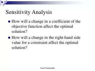
Sensitivity Analysis of Objective Function Coefficients. • Range of Optimality • The optimal solution will remain unchanged as long as • An objective function coefficient lies within its range of optimality • There are no changes in any other input parameters. • The value of the objective function will change if the coefficient multiplies a variable whose value is nonzero.
Sensitivity Analysis of Objective Function Coefficients. X2 1000 Max 4X1 + 5X2 Max 3.75X1 + 5X2 Max 8X1 + 5X2 500 Max 2X1 + 5X2 X1 500 800
Sensitivity Analysis of Objective Function Coefficients. X2 1000 Max8X1 + 5X2 Range of optimality: [3.75, 10] (Coefficient of X1) 500 Max 10 X1 + 5X2 Max 3.75X1 + 5X2 X1 400 600 800
Reduced cost Assuming there are no other changes to the input parameters, the reduced cost for a variable Xj that has a value of “0” at the optimal solution is: • The negative of the objective coefficient increase of the variable Xj (-DCj) necessary for the variable to be positive in the optimal solution • Alternatively, it is the change in the objective value per unit increase of Xj. • Complementary slackness At the optimal solution, either the value of a variable is zero, or its reduced cost is 0.
Sensitivity Analysis of Right-Hand Side Values • In sensitivity analysis of right-hand sides of constraints we are interested in the following questions: • Keeping all other factors the same, how much would the optimal value of the objective function (for example, the profit) change if the right-hand side of a constraint changed by one unit? • For how many additional or fewer units will this per unit change be valid?
Sensitivity Analysis of Right-Hand Side Values • Any change to the right hand side of a binding constraint will change the optimal solution. • Any change to the right-hand side of a non-binding constraint that is less than its slack or surplus, will cause no change in the optimal solution.
Shadow Prices • Assuming there are no other changes to the input parameters, the change to the objective function value per unit increase to a right hand side of a constraint is called the “Shadow Price”
The Plastic constraint Maximum profit = $4360 Maximum profit = $4363.4 Production time constraint Shadow Price – graphical demonstration X2 Whenmore plastic becomes available (the plastic constraint is relaxed), the right hand side of the plastic constraint increases. 1000 2X1 + 1x2 <=1001 2X1 + 1x2 <=1000 500 Shadow price = 4363.40 – 4360.00 = 3.40 X1 500
Range of Feasibility • Assuming there are no other changes to the input parameters, the range of feasibility is • The range of values for a right hand side of a constraint, in which the shadow prices for the constraints remain unchanged. • In the range of feasibility the objective function value changes as follows:Change in objective value = [Shadow price][Change in the right hand side value]
The Plastic constraint A new active constraint Range of Feasibility X2 Increasing the amount of plastic is only effective until a new constraint becomes active. 1000 2X1 + 1x2 <=1000 Production mix constraint X1 + X2£ 700 500 This is an infeasible solution Production time constraint X1 500
The Plastic constraint Range of Feasibility X2 Note how the profit increases as the amount of plastic increases. 1000 2X1 + 1x2£1000 500 Production time constraint X1 500
Infeasible solution A new active constraint Range of Feasibility X2 Less plastic becomes available (the plastic constraint is more restrictive). 1000 The profit decreases 500 2X1 + 1X2£ 1100 X1 500
Other Post - Optimality Changes • Addition of a constraint. • Deletion of a constraint. • Addition of a variable. • Deletion of a variable. • Changes in the left - hand side coefficients.
This cell contains the value of the objective function Set Target cell $D$6 Equal To: By Changing cells These cells containthe decision variables $B$4:$C$4 To enter constraints click… All the constraintshave the same direction, thus are included in one “Excel constraint”. $D$7:$D$10 $F$7:$F$10 Using Excel Solver to Find an Optimal Solution and Analyze Results • To see the input screen in Excel click Galaxy.xls • Click Solver to obtain the following dialog box.
This cell contains the value of the objective function Set Target cell $D$6 Equal To: By Changing cells These cells containthe decision variables $B$4:$C$4 Click on ‘Options’ and check ‘Linear Programming’ and‘Non-negative’. Using Excel Solver • To see the input screen in Excel click Galaxy.xls • Click Solver to obtain the following dialog box. $D$7:$D$10<=$F$7:$F$10
Equal To: Using Excel Solver • To see the input screen in Excel click Galaxy.xls • Click Solver to obtain the following dialog box. Set Target cell $D$6 By Changing cells $B$4:$C$4 $D$7:$D$10<=$F$7:$F$10
Using Excel Solver – Optimal Solution Solver is ready to providereports to analyze theoptimal solution.
Another Example: Cost Minimization Diet Problem • Mix two sea ration products: Texfoods, Calration. • Minimize the total cost of the mix. • Meet the minimum requirements of Vitamin A, Vitamin D, and Iron.
Cost Minimization Diet Problem • Decision variables • X1 (X2) -- The number of two-ounce portions of Texfoods (Calration) product used in a serving. • The Model Minimize 0.60X1 + 0.50X2 Subject to 20X1 + 50X2 ³ 100 Vitamin A 25X1 + 25X2 ³ 100 Vitamin D 50X1 + 10X2 ³ 100 Iron X1, X2 ³ 0 Cost per 2 oz. % Vitamin A provided per 2 oz. % required
The Diet Problem - Graphical solution 10 The Iron constraint Feasible Region Vitamin “D” constraint Vitamin “A” constraint 2 4 5
Cost Minimization Diet Problem • Summary of the optimal solution • Texfood product = 1.5 portions (= 3 ounces) Calration product = 2.5 portions (= 5 ounces) • Cost =$ 2.15 per serving. • The minimum requirement for Vitamin D and iron are met with no surplus. • The mixture provides 155% of the requirement for Vitamin A.