Download
1 / 45
450 likes | 587 Views
Function Learning and Neural Nets R&N: Chap. 20, Sec. 20.5. f(x). x. Function-Learning Formulation. Goal function f Training set: ( x (i) ,y (i) ), i = 1,…,n, y (i) = f ( x (i) ) Inductive inference: find a function h that fits the points well Same Keep-It-Simple bias. f(x). x.

E N D
f(x) x Function-Learning Formulation • Goal function f • Training set: (x(i),y(i)), i = 1,…,n, y(i)=f(x(i)) • Inductive inference: find a function h that fits the points well • Same Keep-It-Simple bias
f(x) x Least-Squares Fitting • Propose a class of functions g(x,q) parameterized by q • Minimize E(q) = Si ( g(x(i),q)-y(i))2
Linear Least-Squares • g(x,q) = x1 q1 + … + xN qN • Best q given byq = (ATA)-1 AT b • Where A is matrix of x(i)’s, b is vector of y(i)’s f(x) g(x,q) x
Constant offset • Set x0=1, g(x,q) = x0 q0 + x1 q1 + … + xN qN • Best q given byq = (ATA)-1 AT b • Where A is matrix of x(i)’s, b is vector of y(i)’s f(x) g(x,q) x
Nonlinear Least-Squares • E.g. quadratic g(x,q) = q0 + xq1 + x2q2 • E.g. exponential g(x,q) = exp(q0 + xq1) • Any combinations g(x,q) = exp(q0 + xq1) + q2 + xq3 quadratic other f(x) linear x
Performance of Nonlinear Least-squares • Overfitting: too many parameters • Efficient optimization • Often can only find a local minimum of objective E(q) • Expensive with lots of data!
Neural Networks • Overfitting: too many parameters • Efficient optimization • Often can only find a local minimum of objective E(q) • Expensive with lots of data!
x2 + + x1 + - + - - S xi y x1 wi + g - - xn y = g(Si=1,…,nwi xi) Perceptron(The goal function f is a boolean one) w1 x1 + w2 x2 = 0
+ + x1 + - - - S xi y wi g - + + - xn y = g(Si=1,…,nwi xi) Perceptron(The goal function f is a boolean one) ?
x1 xi y wi g S xn Unit (Neuron) y = g(Si=1,…,nwi xi) g(u) = 1/[1 + exp(-au)]
x1 xi y wi g S xn A Single Neuron can learn A disjunction of boolean literals x1 x2 x3 Majority function XOR?
x1 x1 S S xi xi y y wi wi g g xn xn Neural Network Network of interconnected neurons Acyclic (feed-forward) vs. recurrent networks
Inputs Hidden layer Output layer Two-Layer Feed-Forward Neural Network w1j w2k
Backpropagation (Principle) • New example y(k) = f(x(k)) • φ(k) = outcome of NN with weights w(k-1) for inputs x(k) • Error function: E(k)(w(k-1)) = ||φ(k) – y(k)||2 • wij(k) = wij(k-1) – εE(k)/wij (w(k) = w(k-1) - eE) • Backpropagation algorithm:Update the weights of the inputs to the last layer, then the weights of the inputs to the previous layer, etc.
Understanding Backpropagation • Minimize E(q) • Gradient Descent… E(q) q
Understanding Backpropagation • Minimize E(q) • Gradient Descent… E(q) Gradient of E q
Understanding Backpropagation • Minimize E(q) • Gradient Descent… E(q) Step ~ gradient q
Understanding Backpropagation • Example of Stochastic Gradient Descent • Minimize E(q) = e1(q)+e2(q)+…+eN(q) • Here ei = (g(x(i),q)-y(i))2 • Take a step to reduce ei E(q) Gradient of e1 q
Understanding Backpropagation • Example of Stochastic Gradient Descent • Minimize E(q) = e1(q)+e2(q)+…+eN(q) • Here ei = (g(x(i),q)-y(i))2 • Take a step to reduce ei E(q) Gradient of e1 q
Understanding Backpropagation • Example of Stochastic Gradient Descent • Minimize E(q) = e1(q)+e2(q)+…+eN(q) • Here ei = (g(x(i),q)-y(i))2 • Take a step to reduce ei E(q) Gradient of e2 q
Understanding Backpropagation • Example of Stochastic Gradient Descent • Minimize E(q) = e1(q)+e2(q)+…+eN(q) • Here ei = (g(x(i),q)-y(i))2 • Take a step to reduce ei E(q) Gradient of e2 q
Understanding Backpropagation • Example of Stochastic Gradient Descent • Minimize E(q) = e1(q)+e2(q)+…+eN(q) • Here ei = (g(x(i),q)-y(i))2 • Take a step to reduce ei E(q) Gradient of e3 q
Understanding Backpropagation • Example of Stochastic Gradient Descent • Minimize E(q) = e1(q)+e2(q)+…+eN(q) • Here ei = (g(x(i),q)-y(i))2 • Take a step to reduce ei E(q) Gradient of e3 q
Stochastic Gradient Descent • Parameter values over time q (local) minimum of E q
Stochastic Gradient Descent • Objective function values over time
Caveats • Choosing a convergent “learning rate” e can be hard in practice E(q) q
Comments and Issues • How to choose the size and structure of networks? • If network is too large, risk of over-fitting (data caching) • If network is too small, representation may not be rich enough • Role of representation: e.g., learn the concept of an odd number • Incremental learning
Role of Marketing • Not a good model of a neuron • Spiking behavior, recurrence in real NNs • No special properties above other learning techniques • Like other learning techniques, a convenient way to get results without thinking too hard
Incremental (“Online”) Function Learning • Data is streaming into learnerx1,y1, …, xt,yt yi = f(xi) • Observes xt+1and must make prediction for next time step yt+1 • Brute force approach: • Store all data at step t • Use your learner of choice on all data up to time t, predict for time t+1
Example: Mean Estimation • yi = q + error term (no x’s) • Current estimate qt= 1/t Si=1…t yi • qt+1= 1/(t+1) Si=1…t+1 yi = 1/(t+1) (yt+1 + Si=1…t yi) = 1/(t+1) (yt+1 + tqt) q5
Example: Mean Estimation • yi = q + error term (no x’s) • Current estimate qt= 1/t Si=1…t yi • qt+1= 1/(t+1) Si=1…t+1 yi = 1/(t+1) (yt+1 + Si=1…t yi) = 1/(t+1) (yt+1 + tqt) y6 q5
Example: Mean Estimation • yi = q + error term (no x’s) • Current estimate qt= 1/t Si=1…t yi • qt+1= 1/(t+1) Si=1…t+1 yi = 1/(t+1) (yt+1 + Si=1…t yi) = 1/(t+1) (yt+1 + tqt) q5 q6 = 5/6 q5 + 1/6 y6
Example: Mean Estimation • qt+1= 1/(t+1) (yt+1 + tqt) • Only need to store t, qt • Similar formulas for standard deviation q5 q6 = 5/6 q6 + 1/6 y6
Incremental Least Squares • Recall Least Squares estimateq = (ATA)-1 AT b • Where A is matrix of x(i)’s, b is vector of y(i)’s (laid out in rows) NxM Nx1 x(1) y(1) x(2) y(2) A = b = … … x(N) y(N)
Incremental Least Squares • Let A(t), b(t) be A matrix, b vector up to time tq(t) = (A(t)TA(t))-1 A(t)T b(t) (T+1)xM (t+1)x1 A(t+1) = A(t) b(t+1) = b(t) x(t+1) y(t+1)
Incremental Least Squares • Let A(t), b(t) be A matrix, b vector up to time tq(t+1) = (A(t+1)TA(t+1))-1 A(t+1)T b(t+1) • A(t+1)T b(t+1) =A(t)T b(t) + y(t+1)x(t+1) (T+1)xM (t+1)x1 A(t+1) = A(t) b(t+1) = b(t) x(t+1) y(t+1)
Incremental Least Squares • Let A(t), b(t) be A matrix, b vector up to time tq(t+1) = (A(t+1)TA(t+1))-1 A(t+1)T b(t+1) • A(t+1)T b(t+1) =A(t)T b(t) + y(t+1)x(t+1) • A(t+1)TA(t+1) = A(t)TA(t) + x(t+1)x(t+1)T (T+1)xM (t+1)x1 A(t+1) = A(t) b(t+1) = b(t) x(t+1) y(t+1)
Incremental Least Squares • Let A(t), b(t) be A matrix, b vector up to time tq(t+1) = (A(t+1)TA(t+1))-1 A(t+1)T b(t+1) • A(t+1)T b(t+1) =A(t)T b(t) + y(t+1)x(t+1) • A(t+1)TA(t+1) = A(t)TA(t) + x(t+1)x(t+1)T (T+1)xM (t+1)x1 A(t+1) = A(t) b(t+1) = b(t) x(t+1) y(t+1)
Incremental Least Squares • Let A(t), b(t) be A matrix, b vector up to time tq(t+1) = (A(t+1)TA(t+1))-1 A(t+1)T b(t+1) • A(t+1)T b(t+1) =A(t)T b(t) + y(t+1)x(t+1) • A(t+1)TA(t+1) = A(t)TA(t) + x(t+1)x(t+1)T • Sherman-Morrison Update • (Y + xxT)-1 = Y-1 - Y-1xxT Y-1 / (1 – xT Y-1 x)
Incremental Least Squares • Putting it all together • Store p(t) = A(t)Tb(t) Q(t) = (A(t)TA(t))-1 • Update p(t+1) = p(t) + y x Q(t+1) = Q(t) - Q(t)xxT Q(t) / (1 – xT Q(t) x)q(t+1) = Q(t+1)p(t+1)
Recap • Function learning with least squares • Neural nets, backpropagation, and gradient descent • Incremental learning
Reminder • HW6 due • HW7 available on Oncourse
Machine Learning Classes • CS659 (Hauser) Principles of Intelligent Robot Motion • CS657 (Yu) Computer Vision • STAT520 (Trosset) Introduction to Statistics • STAT682 (Rocha) Statistical Model Selection