Download
1 / 27
570 likes | 2.05k Views
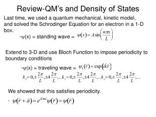
Review-QM’s and Density of States. Last time, we used a quantum mechanical, kinetic model, and solved the Schrodinger Equation for an electron in a 1-D box. - (x) = standing wave = . Extend to 3-D and use Bloch Function to impose periodicity to boundary conditions

E N D
Review-QM’s and Density of States Last time, we used a quantum mechanical, kinetic model, and solved the Schrodinger Equation for an electron in a 1-D box. -(x) = standing wave = Extend to 3-D and use Bloch Function to impose periodicity to boundary conditions -(x) = traveling wave = We showed that this satisfies periodicity. -
Review-QM’s and Density of States Plug into H = E to find energy. Since k, higher energy corresponds to larger k. For kFx=kFy=kFz (i.e. at the Fermi Wave Vector), the Fermi Surface (surface of constant energy, wave vector, temperature) the is a shpere. This applies to valence band for Si, Ge, GaAs; and couduction band for GaAs. • < F, filled states • > F, empty states
If kxF≠kFy≠kFz, then you get constant energy ellipsoids. Also, if k=0 is not lowest energy state, (e.g. for pz orbitals where k= is the lowest energy), you don’t get a constant energy sphere. Fermi Surfaces in Real Materials e.g. Silicon and Germanium CB energy min occurs at Si - X point, k= along <100> directions Ge - L point, k= along <111> directions
Review-QM’s and Density of States # of states in sphere = # of electrons = 2x Number of states, because of spin degeneracy (2 electrons per state) Now we wish to calculate density of states by differentiating N with respect to energy
Review-QM’s and Density of States Number of electrons, n, can be calculated at a given T by integration.
Review-QM’s and Density of States Eff. DOS CB Eff. DOS VB We can now calculate the n,p product by multiplying the above equations. =(intrinsic carrier concentration)2 For no doping and no electric fields Add a field and n≠p, but np=constant
Outline - Moving On Finish up Si Crystal without doping Talk about effective mass, m* Talk about doping Charge Conduction in semiconductors
Intrinsic Semiconductors It is useful to define the “intrinsic Fermi-Level”, what you get for undoped materials. (EF(undoped) = Ei, n=p=ni)
Intrinsic Semiconductors The energy offset from the center of the band gap is in magnitude compared to the magnitude of the bandgap. REMEMBER: There are no states at Ei or EF. They are simply electrochemical potentials that give and average electron energy
Intrinsic Semiconductors For Si and Ge, me* > mh*, so ln term < 0, Ei < Eg For GaAs, me* < mh*, so ln term < 0, Ei < Eg
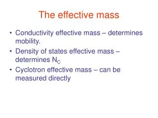
Effective Mass The text book 3.2.4 derives m* from QM treatment of a wave packet. (This expression can be derived quantum mechanically for a wavepacket with group velocity vg) We can use this quantum mechanical results in Newtonian physics. (i.e. Newton’s Secone Law) Thus, electrons in crystals can be treated like “billiard balls” in a semi-classical sense, where crystal forces and QM properties are accounted for in the effective mass.
Effective Mass or So, we see that the effective mass is inversely related to the band curvature. Furthermore, the effective mass depends on which direction in k-space we are “looking” In silicon, for example Where ml* is the effective mass along the longitudinal direction of the ellispoids and mt* is the effective mass along the transverse direction of the ellipsoids
Relative sizes of ml* and mt* are important (ultimately leading to anisotropy in the conductivity) Effective Mass or Again, we stress that effective mass is inversly proportional to band curvature. This means that for negative curvature, a particle will have negative mass and accelerate in the direction opposite to what is expected purely from classical considerations.
One way to measure the effective mass is cyclotron resonance v. crystallographic direction. -We measure the absorption of radio frequency energy v. magnetic field strength. Effective Mass Put the sample in a microwave resonance cavity at 40 K and adjust the rf frequency until it matches the cyclotron frequency. At this point we see a resonant peak in the energy absorption.
Carrier Statistics in Semiconductors Doping -Replace Si lattice atoms with another atom, particularly with an extra or deficient valency. (e.g. P, As, S, B in Si) εD is important because it tells you what fraction of the dopant atoms are going to be ionized at a given temperature. For P in Si, εD = 45 meV, leading to 99.6% ionization at RT. Then, the total electron concentration (for and n type dopant) is
Carrier Statistics in Semiconductors If we look at the Fermi Level position as a function of temperature (for some sample), we see that all donor states are filled at T = 0 (n ≈ 0, no free carriers), EF = ED. At high temperatures, such that, ni >> ND, then n ≈ ni and EF ≈ Ei. EF ranges between these limiting values at intermediate temperatures. (see fig) Np=ni2 still holds, but one must substitute n = ni + ND+ p = ni2/(ni + ND+). At room temperature n ≈ ND+ For Silicon - ni = 1010 cm-3. - ND = 1013→ 1016cm-3 (lightly doped → heavily doped)
Carrier Statistics in Semiconductors This is 60meV/decade. Three decades x 60 meV/decade = 180 meV = EC – EF. EF is very close to the conduction band edge. Similar to EF(T), let’s look at n(T)
Charge Conduction in Semiconductors 1-D 3-D (from Statistical Mechanics) Brownian Motion Applying a force to the particle directionalizes the net movement. The force is necessary since Brownian motion does not direct net current. q < 0 for e-, q > 0 for h+ Constant Field leads to an acceleration of carriers scaled by me*. If this were strictly true, e-’s would accelerate without bound under a constant field. Obviously, this isn’t the case. Electrons are slowed by scattering events.
Scattering Processes in Semiconductors • Ionized Impurity Scattering • Phonon (lattice) Scattering • Neutral Impurity Scattering • Carrier-Carrier Scattering • Piezoelectric Scattering
Scattering Processes in Semiconductors 3) - Donors and acceptors under freez-out. - Low T only - Defect = polycrystalline Si 4) - e- - h+ scattering is insignificant due to low carrier concentration of one type or another - e- - e- or h+ - h+ don’t change mobility since collisions between these don’t change the total momentum of those carriers. 5) - GaAs: displacement of atoms → internal electric field, but very weak. 2) - collisions between carriers and thermally agitated lattice atoms. Acoustic - Mobility decreases as temperature increases due to increased lattice vibration - Mobility decreases as effective mass increases.
Scattering Processes in Semiconductors 1) Coloumb attraction or repulsion between charge carriers and ND+ or NA-. Due to all of these scattering processes, it is possible to define a mean free time, m, and a mean free path lm. Average directed velocity For solar cells (and most devices) high mobility is desirable since you must apply a smaller electric field to move carriers at a give velocity.
Current Flow in Semiconductors e- (cm-3)(cm/s) = e-/cm-2 s A/cm-2 = C/cm-2 s
Resistance n-type For Holes Total Current Flow in Semiconductors