Download
1 / 9
90 likes | 228 Views
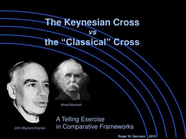
The Keynesian Cross vs the “Classical” Cross. Alfred Marshall. A Telling Exercise in Comparative Frameworks. John Maynard Keynes. Roger W. Garrison 2010. Y = E.

E N D
The Keynesian Cross vs the “Classical” Cross Alfred Marshall A Telling Exercise in Comparative Frameworks John Maynard Keynes Roger W. Garrison 2010
Y = E Expenditures on the economy’s output become the income paid to workers and to other factors of production. “Y = E” constitutes all possible circular-flow equilibria. Spending on consumption goods is a stable function of income. The linear relationship allows for some consumption (“a”) even when income is (temporarily) zero. In a wholly private economy, the only other component of spending is investment spending (“I”), which is simply added vertically to consumption spending (“C”) to get total spending (“E”). Combining “Y=E” with “E=C+I” and taking into account C’s relationship with Y allows us to calculate this economy’s equilibrium income. The primary playing field for Keynesian macroeconomics has the dimensions of INCOME (Y) and EXPENDITURES (E). a = 2,000 b = 0.75 I = 1,250 The intersection of “E=C+I” with “Y=E” (the 450 line allowing income to be measured vertically as well as horizontally) identifies the circular-flow equilibrium point for this particular economy. E = C + I EXPENDITURES C = a + bY 1 b 1 1 Y = E and E = C + I So, Y = C + I, where C = a + bY Combining: Y = a + bY + I Suppose that a = 2,000; b = 0.75; and I = 1,250. I An upward slope (“b”) that is less than one means that when people earn more income, they spend more but they save more, too. a Yeq = 13,000 45O INCOME (Y) We can now write: C = 2,000 + 0.75Y And Y = 2,000 + 0.75Y + I,250 Or: Y – 0.75Y = 2,000 + I,250 Simplifying: 0.25Y = 3,250 Finally: Y = 13,000 If dollar magnitudes are in billions of dollars, then equilibrium income is Yeq = $13,000 billion.
Y = E For low levels of income, consumption spending exceeds income; saving in this low range (shown in red) is negative. The income-expenditure graph tracks consumption spending (C) and total spending (C+I) as these magnitudes relate to income. Indirectly, this graph keeps track of saving, too. Saving (S), which simply means not spending some part of income can be written: S = Y – C. Graphically, S is the vertical distance between C and Y. a = 2,000 b = 0.75 I = 1,250 E = C + I EXPENDITURES C = a + bY For higher levels of income, consumption spending is less than income; saving in this range (shown in green) is positive. I a 45O Where red and green meet, saving is neither negative nor positive. People are neither saving nor dissaving. Rather, S = 0 or, equivalently, C = Y. INCOME (Y)
Y = E We’ve seen that the equality of income and expenditures means that the economy is in a circular-flow equilibrium. We can now show that the equality between saving and investment is an alternative condition for a circular-flow equilibrium. First, we track saving (“S”) as it depends on income. The saving function is derived directly from the definition of saving (S = Y – C) and the consumption function (C = a + bY): a = 2,000 b = 0.75 I = 1,250 E = C + I EXPENDITURES C = a + bY The “a” in the upper panel, which is consumption spending with no income, becomes “-a” in the lower panel, which indicates “dissaving.” S = Y – C C = a + bY Combining: S = Y – (a + bY) Distributing: S = Y – a –bY Rearranging: S = – a + Y –bY Factoring: S = –a + (1 –b)Y Now, for what level of Y is S = 0? I The red-green boundary in the upper panel marks the point in the lower panel where saving is zero. S = –a + (1 –b)Y S = –2,000 + (1 –0.75)Y S = –2,000 + 0.25Y S = –2,000 + 0.25Y = 0 –2,000 = –0.25Y Y = 20/0.25 = 8,000 a 45O INCOME (Y) We now connect the (negative) level of saving when Y=0 and the level of income when S=0 to depict the saving function. SAVIING (S) INVESTMENT (I) S = –a + (1 –b)Y S YS=0 = 8,000 [YS=0); S =0] INCOME (Y) – a 1-b [Y = 0; S =–a] 1
Y = E a = 2,000 b = 0.75 I = 1,200 The income ranges of dissaving (red) and saving (green) are more obvious with S graphed by itself. E = C + I EXPENDITURES C = a + bY Now, we show that investment (I) does not depend on income. I We note that the equality of saving and investment occurs at the same level of income at which income equals expenditures. a 45O INCOME (Y) Notice also that all the information contained or implied in the Y=E graph is also contained or implied in the S=I graph. SAVIING (S) INVESTMENT (I) S I I INCOME (Y) – a
THE KEYNESIAN CROSS THE “CLASSICAL” CROSS The Keynesian Cross, featuring the intersection of Y and E or of S and I, is fundamental to Keynesian theory. Its relevance presupposes that labor markets and output markets are dysfunctional and that the interest rate is out of play. The Keynesian Cross stands in contrast to the “Classical” Cross, whose relevance presuppose that markets work. S RATE OF INTEREST SAVIING (S) INVESTMENT (I) S I D I SAVIING (S) INVESTMENT (D) INCOME (Y) I
Keynes argued that the saving curve doesn’t shift. The parameters “a” and “b” don’t change. And that’s good: if saving were to shift upward, income spirals downward until the equilibrium level of saving, once again, equals the unchanged level of investment. Marshall argued that the supply and demand for loanable funds are fully functional. If saving shifts rightward, the interest rate falls, stimulating an increased level of investment. S This is Keynes’s Paradox of Thrift. RATE OF INTEREST SAVIING (S) INVESTMENT (I) S I D SAVIING (S) INVESTMENT (D) INCOME (Y)
We can identify significant similarities and differences between Keynesian theory and classical theory by responding to a few revealing questions. About what?? About what?? There is no need for stimulus packages. The government should get out of the market’s way and let it work. Laissez faire! The interest rate adjusts, moving up or down in response to shortages or surpluses of loanable funds. Yes. The wage rate adjusts, too, in the face of shortages or surpluses of labor. Where did you learn your microeconomics, Maynard? YES YES –with “equilibrium” understood as a balance between loanable funds supplied and demanded. YES…. Just how is this adjustment made in a market economy? Does the market itself bring about a saving-investment equality? Does “equilibrium” entail an equality of saving and investment? Is the equality of saving and investment consistent with maintaining full employment? What should the government do about it? S No. Only by accident or design is this equality consistent with full employment. Income adjusts. The economy spirals up or down until saving is brought in line with investment. The government should design stimulus packages to supplement spending and drive the economy to full employment. YES…. Al, you’re just an old fuddy-duddy! YES YES –with “equilibrium” understood as a balance between income and expenditures. RATE OF INTEREST SAVIING (S) INVESTMENT (I) S I D SAVIING (S) INVESTMENT (D) INCOME (Y)
The Keynesian Cross vs the “Classical” Cross Alfred Marshall A Telling Exercise in Comparative Analytical Frameworks John Maynard Keynes Roger W. Garrison 2010