Download
1 / 22
220 likes | 394 Views
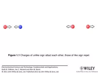
Figure 1.1 Charges of unlike sign attact each other, those of like sign repel. Figure 1.2 The architecture of the dipolar water molecule. The red and blue surface regions are charged positively and negatively respectively.

E N D
Figure 1.1 Charges of unlike sign attact each other, those of like sign repel.
Figure 1.2 The architecture of the dipolar water molecule. The red and blue surface regions are charged positively and negatively respectively.
Figure 1.3 The field created by a positive charge is directed away from the charge in all three-dimensional directions, the converse being true for negative charges.
Figure 1.4 In a spherically symmetrical geometry, all properties are uniform on spheres such as r = R. Here a charge Q resides at the r = 0 origin.
Figure 1.5 The test charge experiences a repulsive force of magnitude Qtestq/2ε from the positively charged sheet, independent of l, and an attractive force of the same magnitude from the negatively charged sheet.
Figure 1.6 A test charge moves a short distance δr from point A to point B towards the source of an electric field. It experiences a field of strength X acting in the direction of increasing r.
Figure 1.7 A test charge journeying by the direct A → B route encounters a field that is constantly changing in both strength and direction. However, the work involved is the same as via the route A → C → B. No work accompanies the A → C journey along the circular arc.
Figure 1.8 Parallel plates store electric charge, and retain the charge when the switch is opened.
Figure 1.9 Measurable potential differences exist within the dielectric and between the metal phases, but not between points in dissimilar phases.
Figure 1.10 In an electric field, dipoles become aligned, to some extent, so that the dipole field opposes the field applied by the plates.
Figure 1.11 Arrangement for measuring the conductivity of an electronic conductor. The method is sometimes called the 4-terminal method because there are four connections to the conductor. The sample of conductor is of length L and cross-sectional area A.
Figure 1.12 In the absence of chemical reaction, current flows transiently when a field is applied to an ionic conductor.
Figure 1.13 How the charge passed varies with time following the imposition of an electric field on three classes of material. For the insulator, a charge of magnitude AεΔE/L passes almost immediately. For the electronic conductor, the charge passed increases linearly as AκtΔE/L. For the ionic conductor, the charge accumulates at an ever-decreasing rate.
Figure 1.14 In the absence of chemical reaction, ions move and accumulate at the interfaces when a field is applied to an ionic conductor.
Figure 1.15 Positive charge carriers move in response to a field, leading to the flow of current I.
Figure 1.16 Cations, moving to the right with the field, and anions, moving leftwards against the field, both contribute to the current.
Figure 1.17 Circuits to evaluate the effect of a voltage step on a resistor and a capacitor in parallel (left) and series (right). In the parallel case, ΔEC and ΔER are identical; when the components are in series, the same current I flows through R and C.
Figure 1.18 How the current changes following the imposition of a constant voltage on a series arrangement of a resistor and a capacitor.
Figure 1.19 Waveforms of the domestic electricity supply: the green and violet curves respectively illustrate 120 V, 60 Hz and 240 V, 50 Hz supplies.
Figure 1.20 An a.c. circuit for measuring the impedance of five alternative loads.
Figure 1.21 A typical Fourier spectrum. In this example, harmonics are present at frequencies of 3ω, 5ω, 7ω, …, in addition to the fundamental of frequency ω. Here,ω = 2π/P.
Figure 1.22 A square wave of amplitude |E|, period P and frequency 2π/P.